2025-04-29 |欢迎您，第位读者！|

Rust for Stupid Engineers愚蠢工程师用Rust

愚蠢工程师用Rust

在考虑用Rust做工程计算——这是一个愚蠢的选择——时，常常需要的一个场景，就是算一大堆数据，然后输出到一个文件中。基本上，我们工程师能够处理的极限就是二维数组，如果是更高维的，我们一个二维数组一个二维数组地处理，毕竟，我们是愚蠢地工程师。

翻开Rust，很好嘛，二维数组：

1let array = [[0; 10]; 10];

这就是一个简单的二维数组，10行10列，每个元素都是0。

简单干净，但是我们只能看不能改。翻翻Rust book（rustup doc --book）。而且，我们是工程师，我们只能处理浮点数。

1let mut array = [[0.0; 10]; 10];
2for i in 0..10 {
3    array[i][i] = 1.0;
4}
5println!("{:?}", array);

打印了我们想要的10维单位矩阵。那么我们工程师是天生懂得复用的。

1fn eye10() -> [[f64; 10]; 10] {
2    let mut array = [[0.0; 10]; 10];
3    for i in 0..10 {
4        array[i][i] = 1.0;
5    }
6    array
7}

现在可以调用这个函数，得到一个10维单位矩阵。

1let array = eye10();
2println!("{:?}", array);

或者，我们要修改这个矩阵，也没问题。当然是很好很强大。

1let mut arr10 = eye10();
2println!("{:?}", arr10);
3
4// arr10[0][0] = 100.00;
5arr10[1][1] = 100.0;
6println!("{:?}", arr10);

总之，不改动的数据，我们用let，要改动的数据，我们用let mut。

数组的使用

当我们把这个处理过程也放在一个函数里面，那要怎么整呢？方案一：输出一个新的二维数组。

1pub fn setij(arr: [[f64; 10]; 10], val: f64, i: usize, j: usize) -> [[f64; 10]; 10] {
2    let mut new_arr = arr;
3    new_arr[i][j] = val;
4    new_arr
5}

用起来也很简单，可以看到，array就是一个值，随便的传递，随便的使用，就跟我们使用普通的1，2，3一样。唯一需要注意的是，我们的数组，大小和类型都是固定的，这个固定的含义是在编译的时候是固定的。这对于工程师来说都不是事情。随便改改Magic number，编译运行，看结果，工程师的快乐就是这么简单。

 1#[test]
 2fn test_set11(){
 3    let arr1 = eye10();
 4    
 5    let (i, j, new_val) = (1, 1, 100.0);
 6    let arr2 = setij(arr1, new_val, i, j);
 7    assert_eq!(arr1[i][j], new_val);
 8    println!("{:?}", arr1);
 9    println!("{:?}", arr2);
10}

哎哎哎，聪（yu）明（chun）的工程师发现了不对，不是说了，arr1被调用了其所有权就被移动了吗？为什么这个也行？那我们还要引用干什么？

1pub fn setij_ref(arr: &[[f64; 10]; 10], val: f64, i: usize, j: usize) -> [[f64; 10]; 10] {
2    let mut new_arr = *arr;
3    new_arr[i][j] = val;
4    new_arr
5}

按照我们的理解，不是应该是这样的吗？完美规避了arr1被移动的问题（我认为！）

但是，array和tuple，以及平凡的简单数据类型：i32, f64, bool, char, 等等，都是Copy的。根本不存在什么所有权被移动的问题。

1let x = 10;
2let y = x;
3println!("x: {}, y: {}", x, y);

这个毫无问题，那谁有问题呢？

1let x = String::from("hello");
2let y = x;
3println!("x: {}, y: {}", x, y);

这个代码就会报错，y=x的时候，字符串的ownership被移动了，只有y能用，x不能用了。

这整个问题就很清楚了，Rust的基本类型（i32, f64, bool, char, 数组，tuple）都是值类型，没有什么所有权，就随便用。而所有权是针对谁的呢？如果学过C语言就知道，是针对堆上的数据。这些值类型，都是放在栈上的，它们的主要特征就是大小在编译的时候就是已知的。那么代价呢，古尔丹？

值数据的代价

对于我们工程师，我们很满意数组可以直接这样用，我们也不在乎需要重新编译程序才能改变数组的大小。在这个层次，我们的Rust程序跟任何其它有GC或者不穿内裤的C语言程序是一样的。

堆栈则无痛。

那么代价呢？我们直接用堆栈就ok，完全不用处理所有权。

代价就是爆栈啊，愚蠢的年轻人。

1#[test]
2fn fuck_stack_with_big_array() {
3    const N : usize = 100000;
4    let array = [[0.0; N]; N];
5    
6}

1cargo test fuck_stack_with_big_array -- --nocapture

程序会输出：thread 'tests::fuck_stack_with_big_array' has overflowed its stack。

实际上，我们可以用stacker这个工具，来查看栈的大小。

1cargo add stacker

1use stacker;
2
3fn main() {
4    println!("Stupidity, and Engineering");
5    let size = stacker::remaining_stack().unwrap();
6    println!("reamaining stack:{}", size);
7    println!("Stack: {} kb", size / 1024 );
8}

1cargo run
2# Stupidity, and Engineering
3# reamaining stack:1018016
4# Stack: 994 kb

可以看到，栈的大小是还不到1MB。我看有本书上说有8MB，也还是很容易爆的。

愚蠢的尝试和解药

愚蠢的尝试

首先，我们知道，堆栈好，堆坏。但是，堆栈那么小，我们工程师的那么大，怎么办？我们从Rust the language book看到，Box就相当于是指针，放在堆上的。马上就动手：

 1#[test]
 2fn test_big_array_usage() {
 3    const N: usize = 1024;
 4    let mut rng = rand::rng();
 5    let mut array = Box::new([[0.0; N]; N]);
 6    for i in 0..N {
 7        for j in 0..N {
 8            array[i][j] = rng.random_range(1.0..100.0);
 9        }
10    }
11
12    assert_eq!(array.len(), N);
13    assert_eq!(array[0].len(), N);
14}

1cargo test test_big_array_usage -- --nocapture

结果就是：thread 'tests::test_big_array_usage' has overflowed its stack。原来，Rust会先在堆栈上创建一个array，然后Copy这个array到堆上，谁让array是值类型呢……

更加愚蠢的`unsafe`领域

那怎么办？我们怎么在堆上面创建一个数组？

 1use std::alloc::alloc;
 2use core::{alloc::Layout, ptr::NonNull};
 3
 4fn heap_array<T, const N: usize>() -> Box<[T; N]> {
 5    unsafe {
 6        let layout = Layout::new::<[T; N]>();
 7        let pointer = alloc(layout);
 8
 9        if pointer.is_null() {
10            panic!("allocation failed");
11        } else{
12            let ptr = NonNull::new_unchecked(pointer as *mut [T; N]);
13            Box::from_raw(ptr.as_ptr())
14        }
15    }
16}

大概就是这样一坨东西，没人希望看懂这个，也没必要看懂这个，工程师懂个屁的编程。

那怎么办？

`vec!`和`Vec<T>`

Rust提供了很好用的动态数组，Vec<T>，还有一个宏实现的语法糖vec!。

1let array = vec![[0.0; N]; N];

对这个这个玩意，我们就需要小心翼翼地处理其所有权转移。

但是工程师搞不了那么复杂地，我们就这样，看看这里，这里的N都不用编译期固定，是一个普通的变量。

 1fn rand_array(array: &mut Vec<Vec<f64>>, rng: &mut impl Rng) {
 2    for i in 0..array.len() {
 3        for j in 0..array[i].len() {
 4            array[i][j] = rng.random_range(1.0..100.0);
 5        }
 6    }
 7}
 8#[test]
 9fn test_very_big_vec() {
10    let N = 8 * 1024 * 1024; // 8 MB
11    let mut rng = rand::rng();
12
13    let mut array = vec![vec![0.0; N]; 2];
14
15    rand_array(&mut array, &mut rng);
16
17    assert_eq!(array.len(), 2);
18    assert_eq!(array[0].len(), N);
19    assert!(array[0].iter().all(|&x| x >= 1.0 && x < 100.0));
20}

我们其实不用管那么多，我们只是按照以下原则：

参数不修改，用&
参数需要修改，用&mut。

所以我们先不管，申明函数写array: &Vec<Vec<f64>>，调用函数写& array，就跟C语言一样，前面是形参，后面是实参。

然后我们cargo check，看看哪里出错，然后我们改成array: &mut Vec<Vec<f64>>和&mut array。

只要从不转移所有权，那么所有权就跟我没有任何关系！

求解简谐振动的ODE

简谐振动

二阶常系数线性微分方程

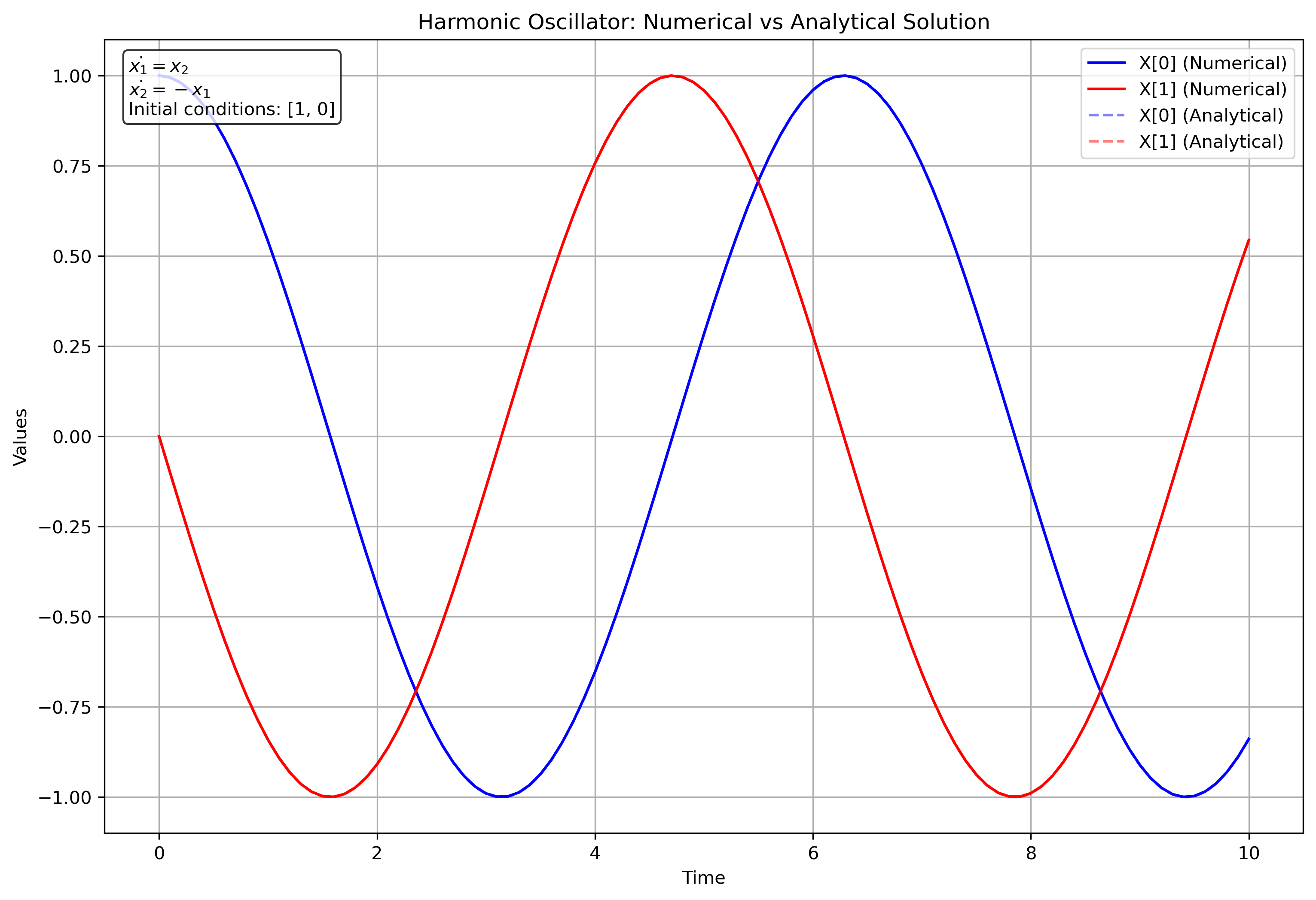
考虑二阶常系数线性微分方程 $x'' = -x$，初始条件为$x(0) = 1$，$x'(0) = 0$。

特征方程求解：
- 设解的形式为 $x(t) = e^{rt}$
- 代入方程得到特征方程：$r^2 + 1 = 0$
- 解得特征根：$r = \pm i$
通解形式：
- 对于复根 $r = \pm i$，通解为： $$x(t) = C_1 \cos(t) + C_2 \sin(t)$$
确定特解：
- 根据初始条件 $x(0) = 1$ 和 $x'(0) = 0$：
  - $x(0) = C_1 = 1$
  - $x'(0) = C_2 = 0$
- 因此特解为：$x(t) = \cos(t)$
- 对应的导数为：$x'(t) = -\sin(t)$
解的物理意义：
- 描述了一个简谐振动
- 振幅为1，周期为 $2\pi$
- 在相空间中形成单位圆：$x^2 + (x')^2 = 1$
验证：
- 二阶导数：$x''(t) = -\cos(t) = -x(t)$
- 初始条件：$x(0) = 1$，$x'(0) = 0$

Rust实现

这个方程，可以写成对应的ODE：

$$ \begin{cases} x' = y \\ y' = -x \end{cases} $$

我本来可以实现一个ODE45，但是我就不，我要实现一个Fehlberg的6阶方法。这里定义了一个OdeFunc，注意看，我们的func函数，需要传入t，x，dx。t是时间，x是状态，dx是状态的变化量，并且按照我前面的原则，dx需要是可变的。

1
2pub trait OdeFunc {
3    fn func(&self, t: f64, x: &Vec<f64>, dx: &mut Vec<f64>);
4    fn dimension(&self) -> usize;
5}

针对这个trait，我们实现一个求解的算法。

 1pub fn rk6<F: OdeFunc>(
 2    ode_func: &F,
 3    t0: f64,
 4    t1: f64,
 5    x0: Vec<f64>,
 6    h: f64,
 7) -> Vec<(f64, Vec<f64>)> {
 8    let mut t = t0;
 9    let mut x = x0.clone();
10    let mut trajectory = vec![(t, x.clone())];
11    let n = ode_func.dimension();
12    let mut k1 = vec![0.0; n];
13    let mut k2 = vec![0.0; n];
14    let mut k3 = vec![0.0; n];
15    let mut k4 = vec![0.0; n];
16    let mut k5 = vec![0.0; n];
17    let mut k6 = vec![0.0; n];
18    let mut dx = vec![0.0; n];
19
20    while t < t1 {
21        let h_actual = if t + h > t1 { t1 - t } else { h };
22
23        // 计算 Runge-Kutta 的系数
24        ode_func.func(t, &x, &mut k1);
25        for i in 0..n {
26            dx[i] = x[i] + h_actual * k1[i] / 4.0;
27        }
28        ode_func.func(t + h_actual / 4.0, &dx, &mut k2);
29        for i in 0..n {
30            dx[i] = x[i] + h_actual * (3.0 * k1[i] + 9.0 * k2[i]) / 32.0;
31        }
32        ode_func.func(t + 3.0 * h_actual / 8.0, &dx, &mut k3);
33        for i in 0..n {
34            dx[i] = x[i] + h_actual * (1932.0 * k1[i] - 7200.0 * k2[i] + 7296.0 * k3[i]) / 2197.0;
35        }
36        ode_func.func(t + 12.0 * h_actual / 13.0, &dx, &mut k4);
37        for i in 0..n {
38            dx[i] = x[i] + h_actual * (439.0 * k1[i] / 216.0 - 8.0 * k2[i] + 3680.0 * k3[i] / 513.0 - 845.0 * k4[i] / 4104.0);
39        }
40        ode_func.func(t + h_actual, &dx, &mut k5);
41        for i in 0..n {
42            dx[i] = x[i] + h_actual * (-8.0 * k1[i] / 27.0 + 2.0 * k2[i] - 3544.0 * k3[i] / 2565.0 + 1859.0 * k4[i] / 4104.0 - 11.0 * k5[i] / 40.0);
43        }
44        ode_func.func(t + h_actual / 2.0, &dx, &mut k6);
45
46        // 更新状态
47        for i in 0..n {
48            x[i] += h_actual
49                * (16.0 * k1[i] / 135.0
50                    + 6656.0 * k3[i] / 12825.0
51                    + 28561.0 * k4[i] / 56430.0
52                    - 9.0 * k5[i] / 50.0
53                    + 2.0 * k6[i] / 55.0);
54        }
55        t += h_actual;
56        trajectory.push((t, x.clone()));
57    }
58
59    trajectory
60}

然后在main函数中，我们就可以这样使用：

 1use rust_for_stupid_engineers::ode::{rk6, OdeFunc};
 2
 3struct SimpleOde {
 4    dim: usize,
 5}
 6
 7impl OdeFunc for SimpleOde {
 8    fn func(&self, _t: f64, x: &Vec<f64>, dx: &mut Vec<f64>) {
 9        dx[0] = x[1];
10        dx[1] = -x[0];
11    }
12
13    fn dimension(&self) -> usize {
14        self.dim
15    }
16}
17
18fn main() {
19    let ode = SimpleOde { dim: 2 };
20    let t0 = 0.0;
21    let t1 = 10.0;
22    let x0 = vec![1.0, 0.0];
23    let h = 0.1;
24
25    let result = rk6(&ode, t0, t1, x0, h);
26
27    println!("#{}", "ODE45 Result");
28    println!("#{:<18}{:<18}{:<18}", "Time", "X[0]", "X[1]");
29    for (t, x) in result {
30        println!("{:<18.4}{:<18.4}{:<18.4}", t, x[0], x[1]);
31    }
32}

最后整个脚本把数据画出来：

 1import matplotlib.pyplot as plt
 2import numpy as np
 3import os
 4
 5
 6def read_results(file_path):
 7    """Reads the results file and extracts time, X[0], and X[1]."""
 8    time = []
 9    x0 = []
10    x1 = []
11    with open(file_path, 'r', encoding='utf-8', errors='ignore') as file:
12        for line in file:
13            if line.startswith("#") or not line.strip():
14                continue  # Skip comments and empty lines
15            # Clean the line of any non-printable characters
16            line = ''.join(char for char in line if char.isprintable())
17            parts = line.split()
18            if len(parts) >= 3:  # Ensure we have at least 3 values
19                try:
20                    time.append(float(parts[0]))
21                    x0.append(float(parts[1]))
22                    x1.append(float(parts[2]))
23                except ValueError:
24                    continue  # Skip lines that can't be converted to float
25    return time, x0, x1
26
27
28def analytical_solution(t):
29    """Returns the analytical solution for the ODE system."""
30    # x1(t) = cos(t)
31    # x2(t) = -sin(t)
32    return np.cos(t), -np.sin(t)
33
34
35def plot_results(time, x0, x1, save_path=None):
36    """Plots X[0] and X[1] against time."""
37    plt.figure(figsize=(12, 8))
38
39    # Plot numerical solution
40    plt.plot(time, x0, label="X[0] (Numerical)", color="blue", linestyle='-')
41    plt.plot(time, x1, label="X[1] (Numerical)", color="red", linestyle='-')
42
43    # Plot analytical solution
44    t_analytical = np.linspace(min(time), max(time), 1000)
45    x1_analytical, x2_analytical = analytical_solution(t_analytical)
46    plt.plot(t_analytical, x1_analytical,
47             label="X[0] (Analytical)", color="blue", linestyle='--', alpha=0.5)
48    plt.plot(t_analytical, x2_analytical,
49             label="X[1] (Analytical)", color="red", linestyle='--', alpha=0.5)
50
51    # Add ODE description
52    ode_text = r"$\dot{x_1} = x_2$" + "\n" + \
53        r"$\dot{x_2} = -x_1$" + "\n" + "Initial conditions: [1, 0]"
54    plt.text(0.02, 0.98, ode_text, transform=plt.gca().transAxes,
55             verticalalignment='top', bbox=dict(boxstyle='round', facecolor='white', alpha=0.8))
56
57    plt.title("Harmonic Oscillator: Numerical vs Analytical Solution")
58    plt.xlabel("Time")
59    plt.ylabel("Values")
60    plt.legend()
61    plt.grid(True)
62
63    if save_path:
64        plt.savefig(save_path, dpi=300, bbox_inches='tight')
65        print(f"Plot saved to {save_path}")
66    else:
67        plt.show()
68
69
70if __name__ == "__main__":
71    # Get the directory of the current script
72    script_dir = os.path.dirname(os.path.abspath(__file__))
73    # Go up one directory to find the results file
74    results_dir = os.path.dirname(script_dir)
75    results_file = os.path.join(results_dir, "results")
76    time, x0, x1 = read_results(results_file)
77    plot_results(time, x0, x1, save_path=os.path.join(
78        results_dir, "results_plot.png"))

还有那个动画脚本：

  1import matplotlib.pyplot as plt
  2import numpy as np
  3from matplotlib.animation import FuncAnimation
  4import os
  5
  6
  7def read_results(file_path):
  8    """Reads the results file and extracts time, X[0], and X[1]."""
  9    time = []
 10    x0 = []
 11    x1 = []
 12    with open(file_path, 'r', encoding='utf-8', errors='ignore') as file:
 13        for line in file:
 14            if line.startswith("#") or not line.strip():
 15                continue
 16            line = ''.join(char for char in line if char.isprintable())
 17            parts = line.split()
 18            if len(parts) >= 3:
 19                try:
 20                    time.append(float(parts[0]))
 21                    x0.append(float(parts[1]))
 22                    x1.append(float(parts[2]))
 23                except ValueError:
 24                    continue
 25    return np.array(time), np.array(x0), np.array(x1)
 26
 27
 28def create_animation(time, x0, x1, save_path):
 29    """Creates an animation of the harmonic oscillator."""
 30    # Create figure with two subplots
 31    fig, (ax1, ax2) = plt.subplots(1, 2, figsize=(12, 6))
 32
 33    # Set up the time series plot
 34    ax1.set_xlim(time[0], time[-1])
 35    ax1.set_ylim(-1.2, 1.2)
 36    ax1.grid(True)
 37    ax1.set_title('Time Series')
 38    ax1.set_xlabel('Time')
 39    ax1.set_ylabel('Value')
 40
 41    # Set up the phase space plot
 42    ax2.set_xlim(-1.2, 1.2)
 43    ax2.set_ylim(-1.2, 1.2)
 44    ax2.set_aspect('equal')
 45    ax2.grid(True)
 46    ax2.set_title('Phase Space')
 47    ax2.set_xlabel('x1')
 48    ax2.set_ylabel('x2')
 49
 50    # Plot the full trajectory in phase space
 51    ax2.plot(x0, x1, 'b-', alpha=0.3, label='Trajectory')
 52
 53    # Initialize the time series lines and phase space point
 54    line1, = ax1.plot([], [], 'b-', label='x1')
 55    line2, = ax1.plot([], [], 'r-', label='x2')
 56    phase_point, = ax2.plot([], [], 'ro', markersize=10)
 57
 58    # Add vertical line for current time
 59    vline = ax1.axvline(x=0, color='k', linestyle='--', alpha=0.5)
 60
 61    # Add legends
 62    ax1.legend()
 63    ax2.legend()
 64
 65    def init():
 66        line1.set_data([], [])
 67        line2.set_data([], [])
 68        phase_point.set_data([], [])
 69        vline.set_xdata([0])
 70        return line1, line2, phase_point, vline
 71
 72    def update(frame):
 73        # Update time series plot
 74        current_time = time[frame]
 75        line1.set_data(time[:frame+1], x0[:frame+1])
 76        line2.set_data(time[:frame+1], x1[:frame+1])
 77        vline.set_xdata([current_time])
 78
 79        # Update phase space point
 80        phase_point.set_data(x0[frame], x1[frame])
 81        return line1, line2, phase_point, vline
 82
 83    # Create animation
 84    anim = FuncAnimation(fig, update, frames=len(time),
 85                         init_func=init, blit=True,
 86                         interval=20)  # 50 fps
 87
 88    # Save animation
 89    anim.save(save_path, writer='pillow', fps=50)
 90    print(f"Animation saved to {save_path}")
 91
 92
 93if __name__ == "__main__":
 94    # Get the directory of the current script
 95    script_dir = os.path.dirname(os.path.abspath(__file__))
 96    # Go up one directory to find the results file
 97    results_dir = os.path.dirname(script_dir)
 98    results_file = os.path.join(results_dir, "results")
 99
100    # Read the results
101    time, x0, x1 = read_results(results_file)
102
103    # Create animation
104    save_path = os.path.join(results_dir, "harmonic_oscillator.gif")
105    create_animation(time, x0, x1, save_path)

总结

其实Rust拿来做计算还是挺方便的。我还没有开始用更加好用的ndarray和相关的线性代数包。

工程师搞什么优雅，能在堆栈上解决，咱们就堆栈解决；实在不行，用Vec<T>解决，然后全部搞不可变引用&Vec<T>，在编译器的指导下把部分地方改成可变引用&mut Vec<T>。