Structural_Transient_In_Matlab结构动力学问题求解
结构动态问题
问题描述
我们试着给前面已经做过的问题上加一点有趣的东西。
当时求解这个问题,在最外面的竖直切面加载了一个静态的固定的力。下面我们试试看在上方的表面增加一个脉冲压力载荷。
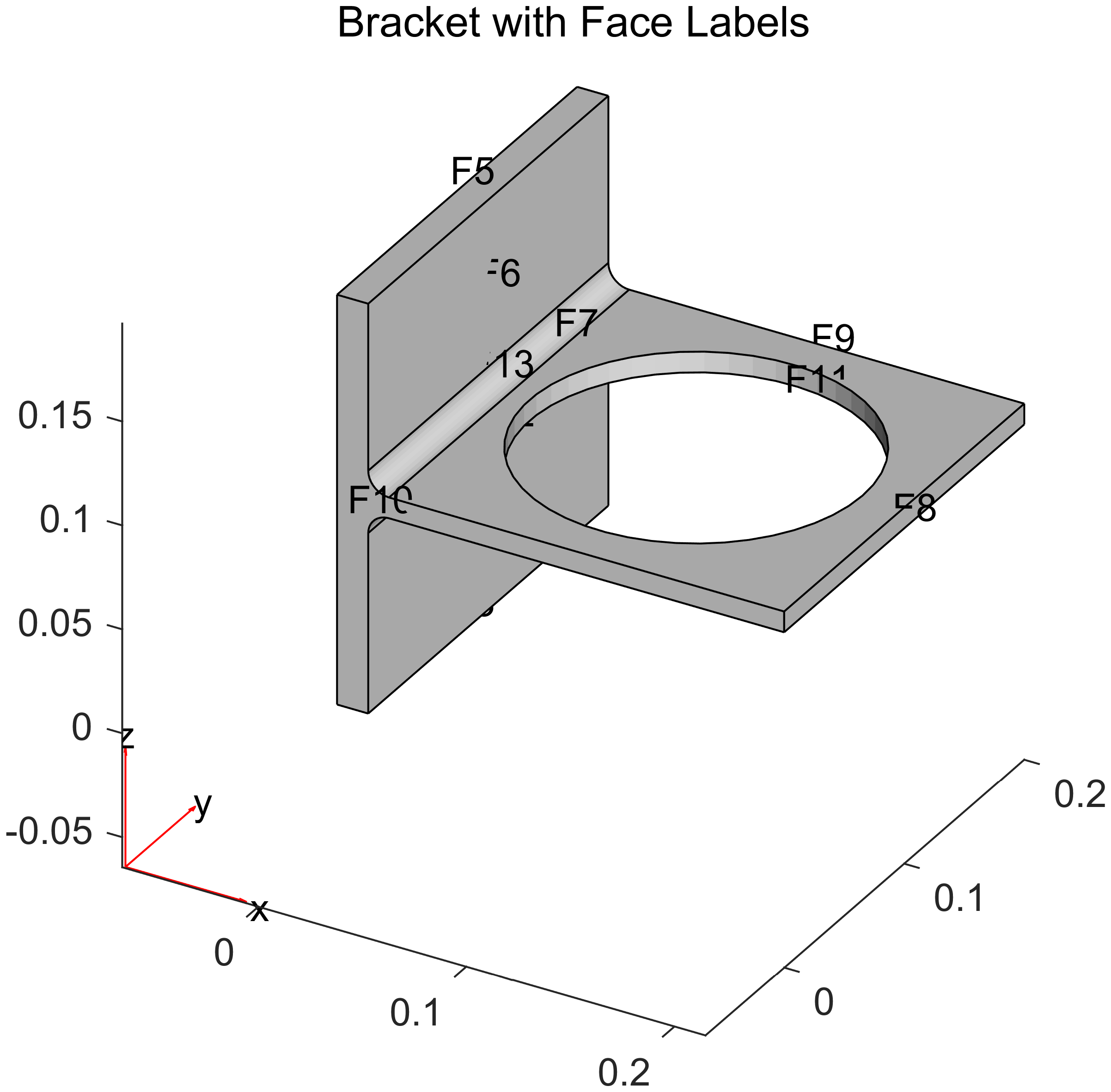
采用统一的有限元框架,定义问题,几何体已经出现过一次。
1%% Rectangular Pressure Pulse on Boundary
2
3% Create a model and include the bracket geometry.
4model = femodel(AnalysisType="structuralTransient", ...
5    Geometry="BracketWithHole.stl");
6
7pdegplot(model.Geometry, 'FaceLabels', 'on', 'FaceAlpha', 0.5);
材料特性设置。
1% Specify Young's modulus, Poisson's ratio, and mass density.
2model.MaterialProperties = ...
3    materialProperties(YoungsModulus=200e9, ...
4    PoissonsRatio=0.3, MassDensity=7800);
边界与加载
边界条件
首先是固定表面,我们把最大的竖直表面固定起来。
1% Specify that face 4 is a fixed boundary.
2model.FaceBC(4) = faceBC(Constraint="fixed");
注意,我们这里设置边界条件的函数,由小写字母开头,而设置好的边界条件的变量,首字母是大写的。通过在faceBC中的Name=Value可以设置边界条件的值。
可以查看faceBC的帮助。
1help faceBC
 faceBC - Boundary conditions on geometry face
    A faceBC object specifies the type of boundary condition on a face of a
    geometry.

    创建
      语法
        model.FaceBC(FaceID) = faceBC(Name=Value)

      输入参数
        FaceID - Face IDs
          vector of positive integers

    属性
      Constraint - Standard structural boundary constraints
        "fixed"
      XDisplacement - x-component of enforced displacement
        real number | function handle
      YDisplacement - y-component of enforced displacement
        real number | function handle
      ZDisplacement - z-component of enforced displacement
        real number | function handle
      Temperature - Temperature boundary condition
        real number | function handle
      Voltage - Voltage
        real number | function handle
      ElectricField - Electric field
        column vector | function handle
      MagneticField - Magnetic field
        column vector | function handle
      MagneticPotential - Magnetic potential
        real number | column vector | function handle
      FarField - Absorbing region
        farFieldBC object

    示例
      openExample('pde/FixedBoundariesExample')
      openExample('pde/BoundaryConditionsFor3DHarmonicElectromagneticAnalysisExample')

    另请参阅 femodel, fegeometry, farFieldBC, edgeBC, vertexBC, cellLoad,
      faceLoad, edgeLoad, vertexLoad

    已在 R2023a 中的 Partial Differential Equation Toolbox 中引入
    faceBC 的文档
       doc faceBC
接下来就是这个比较难的脉冲加载。
加载的设置方法,类似于边界条件的设置。可以设置不同的选择,例如,对于结构问题:
Pressure:垂直于面的压力载荷,单位为PaSurfaceTraction:表面载荷,力,单位为N
1% Apply a rectangular pressure pulse on face 7 in the direction normal to the face.
2pressurePulse = @(location,state) ...
3    rectangularLoad(10^5,location,state,[0.0 0.002]);
4model.FaceLoad(7) = faceLoad(Pressure=pressurePulse);
这里的问题,脉冲载荷如何实现?
脉冲加载
在faceLoad函数的Name=Value中,值可以采取多种形式,主要我们用到的是数值和函数。
当这里使用一个函数是, 对函数的输入和输出有固定的要求。
- 输入1:位置,一般称为
location - 输入2: 状态
1function value = loadFucntion(location, state)
2
3end
这个函数的两个参数分别是位置和状态,是两个结构体,其具体内容如下:
- location — 结构体,包含以下字段::
- location.x — x坐标,是一个点或者若干个点
- location.y — y坐标,是一个点或者若干个点
- location.z — z坐标,是一个点或者若干个点
- location.nx — 法向量的x分量,是一个点的或者若干个点的
- location.ny — 法向量的y分量,是一个点的或者若干个点的
- location.nz — 法向量的z分量,是一个点的或者若干个点的
- state — 对于非线性问题和动态问题才有意义,包括以下字段的结构体:
- state.u — 对应与
location中定义点的状态变量(对于结构问题,就是位移) - state.ux — 估计的导数x分量
- state.uy — 估计的导数y分量
- state.uz — 估计的导数y分量
- state.time — 时间
- state.frequency — 频率
- state.NormFluxDensity — 非线性磁场问题才需要的参数
- state.u — 对应与
对于我们想要求解的脉冲压力载荷问题,我们定义一个方波脉冲,这个方波脉冲的参数包括:
load,载荷大小T,载荷时间,一个数组,包含两个时间点,分别是载荷开始和结束的时间
 1function Tn = rectangularLoad(load,location,state,T)
 2if isnan(state.time)
 3    Tn = NaN*(location.nx);
 4    return
 5end
 6if isa(load,"function_handle")
 7    load = load(location,state);
 8else
 9    load = load(:);
10end
11% Two time-points that define a rectangular pulse
12T1 = T(1); % Start time
13T2 = T(2); % End time
14
15% Determine multiplicative factor for the specified time.
16TnTrap = max([(state.time - T1)*(T2 - state.time)/ ...
17    abs((state.time - T1)*(T2 - state.time)),0]);
18Tn = load.* TnTrap;
19end
最后这个TnTrap是一个方波函数,其值在T1和T2之间为1,其他地方为0。
因为这里我们是一个时变问题,所以用到了state.time,这个是时间。
现在回到我们的设置中:
1pressurePulse = @(location,state) ...
2    rectangularLoad(10^5,location,state,[0.0 0.002]);
我们用上面方波函数定义了一个载荷函数,大小为$10^5$,载荷时间为0到0.002s。
求解
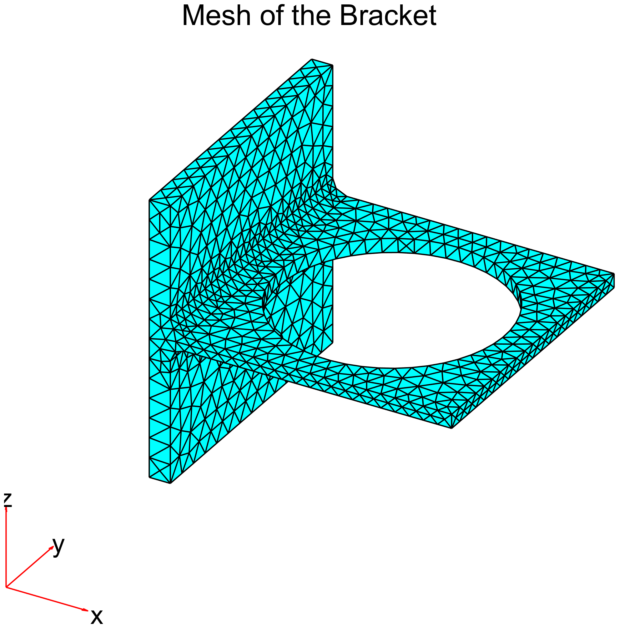
接下来就是网格和求解。
1% Generate a mesh and assign it to the model.
2model = generateMesh(model);
3
4% pdemesh(model);
5
6% 也可以是
7
8pdeplot3D(model.Geometry.Mesh);
求解要针对一个时间序列,这里我们设置时间序列为0到0.01s,取100个点。尽量分辨脉冲的宽度0.002s。
1% Solve the problem.
2result = solve(model,linspace(0,0.01,100));
可视化
前面我们利用pdeplot3D函数进行可视化,这个函数可以把求解的结果映射到网络结构上,对点、线、面进行着色。在前面两个结构静力学的例子中都得到应用。
这里,因为是一个动态问题,我们实际更想要更好地理解在动态载荷下,结构是如何发生变形和位移的。
这里我们就要介绍一个新的函数pdeviz,这个函数提供了更多的可视化功能,可以对结构的变形、位移、应力、应变等进行可视化。
另外,在动态问题的结果中,我们看看,结果包含了哪些内容:
1result
result =

  TransientStructuralResults - 属性:

     Displacement: [1x1 FEStruct]
         Velocity: [1x1 FEStruct]
     Acceleration: [1x1 FEStruct]
    SolutionTimes: [0 1.0101e-04 2.0202e-04 3.0303e-04 4.0404e-04 5.0505e-04 6.0606e-04 7.0707e-04 8.0808e-04 ... ] (1x100 double)
             Mesh: [1x1 FEMesh]
那么我们要用应力来着色,还需要用到一系列专门给输出利用的函数,这些函数都用evaluate开头。
evaluateStress动态结构问题的应力评估evaluateStrain动态结构问题的应变评估evaluateVonMisesStress动态结构问题的von Mises应力评估
此外,还有下面的几个函数:
evaluateReaction评估边界的反作用力evaluatePrincipalStress评估节点位置的主应力evaluatePrincipalStrain评估节点位置的主应变
有上述函数的帮助,我们可以构造一个动态过程的可视化。
 1fn = "structuralDyanmicLoad-viz.gif";
 2if isfile(fn)
 3    delete(fn)
 4end
 5
 6
 7vmStress = evaluateVonMisesStress(result);
 8
 9v = pdeviz(model.Geometry.Mesh);
10v.MeshVisible = "off";
11v.AxesVisible = "on";
12v.DeformationScaleFactor = 10;
13
14for i = 2:numel(result.SolutionTimes)
15    % pdeplot3D(result.Mesh, ColorMapData=result.Displacement.uz(:,i))
16    title(sprintf("Time: %.5f s",result.SolutionTimes(i)))
17
18    v.NodalData = vmStress(:, i);
19    v.DeformationData = ...
20        struct('ux', result.Displacement.ux(:, i), ...
21            'uy', result.Displacement.uy(:, i), ...
22            'uz', result.Displacement.uz(:, i));
23
24    % specificy fixed color limits
25    clim([0, 1e8])
26
27    exportgraphics(gcf, fn, Append=true, Resolution=80)
28end
当然这里的位移是进行整体放大的,v.DeformationScaleFactor = 10;,这个可以调整。
完整代码
完整的代码如下:
 1%% Rectangular Pressure Pulse on Boundary
 2
 3% Create a model and include the bracket geometry.
 4model = femodel(AnalysisType="structuralTransient", ...
 5    Geometry="BracketWithHole.stl");
 6
 7% Specify Young's modulus, Poisson's ratio, and mass density.
 8model.MaterialProperties = ...
 9    materialProperties(YoungsModulus=200e9, ...
10    PoissonsRatio=0.3, MassDensity=7800);
11
12% Specify that face 4 is a fixed boundary.
13model.FaceBC(4) = faceBC(Constraint="fixed");
14
15% By default, both the initial displacement and velocity are set to 0.
16
17% Apply a rectangular pressure pulse on face 7 in the direction normal to the face.
18pressurePulse = @(location,state) ...
19    rectangularLoad(10^5,location,state,[0.0 0.002]);
20model.FaceLoad(7) = faceLoad(Pressure=pressurePulse);
21
22% Generate a mesh and assign it to the model.
23model = generateMesh(model,Hmax=0.05);
24
25% Solve the problem.
26result = solve(model,linspace(0,0.01,100));
27
28
29fn = "structuralDyanmicLoad-viz.gif";
30if isfile(fn)
31    delete(fn)
32end
33
34
35vmStress = evaluateVonMisesStress(result);
36
37v = pdeviz(model.Geometry.Mesh);
38v.MeshVisible = "off";
39v.AxesVisible = "on";
40v.DeformationScaleFactor = 10;
41
42for i = 2:numel(result.SolutionTimes)
43    % pdeplot3D(result.Mesh, ColorMapData=result.Displacement.uz(:,i))
44    title(sprintf("Time: %.5f s",result.SolutionTimes(i)))
45
46    v.NodalData = vmStress(:, i);
47    v.DeformationData = struct('ux', result.Displacement.ux(:, i), ...
48        'uy', result.Displacement.uy(:, i), ...
49        'uz', result.Displacement.uz(:, i));
50
51
52    % specificy fixed color limits
53    clim([0, 1e8])
54
55    exportgraphics(gcf, fn, Append=true, Resolution=80)
56end
文章标签
|-->matlab |-->FEM |-->transient |-->structure
- 本站总访问量:loading次
- 本站总访客数:loading人
- 可通过邮件联系作者:Email大福
- 也可以访问技术博客:大福是小强
- 也可以在知乎搞抽象:知乎-大福
- Comments, requests, and/or opinions go to: Github Repository