2025-05-22 |欢迎您，第位读者！|

Matlab PDE工具箱非均匀材料的处理方式

如何处理非均匀的材料

在Matlab PDE工具箱中，非均匀材料的处理非常简单。这里可以分两种情况来讨论。第一种情况，计算与可以分为多个区域，每个区域有不同的材料属性。第二种情况，计算域中材料属性是连续变化的。

一般而言，用有限元处理的偏微分方程远没有有限差分那么有意思，哦，不对，是没那么恶心。

有限元的复杂，我觉得多半在材料特性上。

按区域设定材料

我们先假设一个传热的例子，计算域中包含两个区域，每个区域有不同的材料属性。

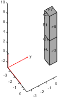
在进行几何建模时，我们就应该分别建立两个几何域来组成计算区域。

C1+C2

1% 几何建模
2length = 10;
3gm = multicuboid([1, 1],[1, 1], [length * 0.5, length * 0.5], 'Zoffset', [0, 0.5*length]);
4
5pdegplot(gm, 'CellLabels', 'on', 'FaceLabels', 'on');
6
7view(57, 56);
8exportgraphics(gcf, 'heatTransferInNonUniformPod.png', 'Resolution', 60);

从这里可以看到，两个Cell（分别是C1和C2）组成了整个计算域。

在材料建模时，我们分别对C1和C2进行材料建模。

1% 材料建模
2material1 = materialProperties("ThermalConductivity", 1, "MassDensity", 1, "SpecificHeat", 1);
3material2 = materialProperties("ThermalConductivity", 100, "MassDensity", 1, "SpecificHeat", 1);
4
5model.MaterialProperties(1) = material1;
6model.MaterialProperties(2) = material2;

在设置完之后，我们可以查看材料属性。

1>> model.MaterialProperties
2ans = 
3  1x2 materialProperties array
4
5Properties for analysis type: thermalTransient
6
7Index    ThermalConductivity    MassDensity    SpecificHeat
8  1               1                  1              1      
9  2              100                 1              1

从这里可以看到，C1和C2的材料属性分别被设置为1和100。

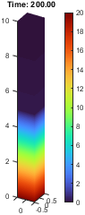
最后，按照正常步骤求解即可。

result

 1% 非均匀材料的热传导问题
 2
 3
 4model = femodel("AnalysisType","thermalTransient");
 5
 6% 几何建模
 7length = 10;
 8gm = multicuboid([1, 1],[1, 1], [length * 0.5, length * 0.5], 'Zoffset', [0, 0.5*length]);
 9
10pdegplot(gm, 'CellLabels', 'on', 'FaceLabels', 'on');
11
12view(57, 56);
13exportgraphics(gcf, 'heatTransferInNonUniformPod.png', 'Resolution', 60);
14
15model.Geometry = gm;
16
17model = generateMesh(model);
18
19pdemesh(model);
20
21% 材料建模
22material1 = materialProperties("ThermalConductivity", 1, "MassDensity", 1, "SpecificHeat", 1);
23material2 = materialProperties("ThermalConductivity", 100, "MassDensity", 1, "SpecificHeat", 1);
24
25model.MaterialProperties(1) = material1;
26model.MaterialProperties(2) = material2;
27
28model.CellIC = cellIC("Temperature", 20);
29
30model.FaceBC(1) = faceBC("Temperature", 20);
31model.FaceBC(7) = faceBC("Temperature", 0);
32
33tspan = linspace(0, 200, 1000);
34result = solve(model, tspan);
35
36% using pdeviz build a animation of the heating process
37
38V = pdeviz(model.Mesh, result.Temperature(:,1));
39V.ColorLimits = [0, 20];
40colorbar;
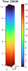
41for ti = 1:numel(tspan)
42    V.NodalData = result.Temperature(:,ti);
43    title(sprintf('Time: %.2f', tspan(ti)));
44    pause(0.001);
45end
46
47exportgraphics(gcf, 'result3.png', 'Resolution', 60);

设置为连续变化的材料

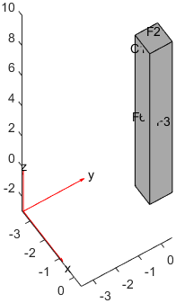
当然还有一种办法，就是采用材料函数来设定，用这个方法，我们在建模时就不需要分别建立几何域了。

1% 几何建模
2length = 10;
3gm = multicuboid(1, 1, length);
4
5pdegplot(gm, 'CellLabels', 'on', 'FaceLabels', 'on');
6
7view(57, 56);
8exportgraphics(gcf, 'singleCell.png', 'Resolution', 100);

result

我们的材料属性函数（准确来说是材料导热系数）是一个函数句柄，这个函数句柄的输入参数是位置和状态，输出参数是材料导热系数。

1function k = k_func(location, ~)
2k = 9.9 * location.z + 1;
3end

这就是一个1.0到100的线性函数。

result

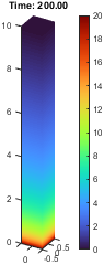
最后的计算结果跟两段材料大相径庭。全部代码：

 1% 非均匀材料的热传导问题
 2
 3
 4model = femodel("AnalysisType","thermalTransient");
 5
 6% 几何建模
 7length = 10;
 8gm = multicuboid(1, 1, length);
 9
10pdegplot(gm, 'CellLabels', 'on', 'FaceLabels', 'on');
11
12view(57, 56);
13exportgraphics(gcf, 'singleCell.png', 'Resolution', 100);
14
15model.Geometry = gm;
16
17model = generateMesh(model);
18
19pdemesh(model);
20
21% 材料建模
22% k = @(location, state) 9.9 * location.z + 1;
23
24model.MaterialProperties = materialProperties(...
25    "ThermalConductivity", @k_func,...
26    "MassDensity", 1,...
27    "SpecificHeat", 1);
28
29model.CellIC = cellIC("Temperature", 20);
30
31model.FaceBC(1) = faceBC("Temperature", 20);
32model.FaceBC(2) = faceBC("Temperature", 0);
33
34tspan = linspace(0, 200, 1000);
35result = solve(model, tspan);
36
37% using pdeviz build a animation of the heating process
38
39V = pdeviz(model.Mesh, result.Temperature(:,1));
40V.ColorLimits = [0, 20];
41colorbar;
42for ti = 1:numel(tspan)
43    V.NodalData = result.Temperature(:,ti);
44    title(sprintf('Time: %.2f', tspan(ti)));
45    pause(0.001);
46end
47
48exportgraphics(gcf, 'result2.png', 'Resolution', 60);
49
50function k = k_func(location, ~)
51k = 9.9 * location.z + 1;
52end

如果我们算一个热导率全部取为100的，结果会怎么样？

result

只能说，传热还是有那么一点点意思的……

总结

我优先会选择按照多个域方式来进行处理，实在不行采取采取第二种方式，第二种方式的计算可能会不收敛，需要精心处理网格和时间步长。

当然这个方法实际上可以用于所有的边界条件、初始条件、材料属性。

对于大部分参数，通用的方式就是：

1function val = myfun(location, state)
2    val = ...;
3end

而对于初始温度、初始位移或者初始速度，函数变为：

1function val = myfun(location)
2    val = ...;
3end

这个函数的输入阐述通常是一个结构体数组，可以自行探索在不同的计算中，具体的结构体数组是什么样的。