Non-stiff ODE在MATLAB中非刚性ODE求解
Rayleigh方程
Rayleigh ODE是一个经典的非线性微分方程,通常用于描述振动和波动现象。它的形式为:
$$ y'' - \mu (1-\frac{1}{3}y'^2)y' + y = 0 \tag{1} $$或者,其中的$\frac{1}{3}y'^2$被替换为1的方程也有时候被称为Rayleigh方程。
$$ y'' - \mu (1-y'^2)y' + y = 0 $$我们这里,还是按照第一种形式来讨论。
如果我们把式(1)取导数可以得到:
$$ y''' - \mu (1 - y'^2)y'' + y' = 0 \tag{2} $$我们把式(2)中的$y'$替换为$y$,得到:
$$ y'' - \mu (1- y^2) y' + y = 0 \tag{3} $$这个方程通常被称为von der Pol方程。
考虑到Rayleigh方程的物理含义是单簧管簧片的速度非线性阻尼的振动方程(振动位移为因变量$y$),von der Pol方程的物理含义是以振动速度为因变量的振动方程。
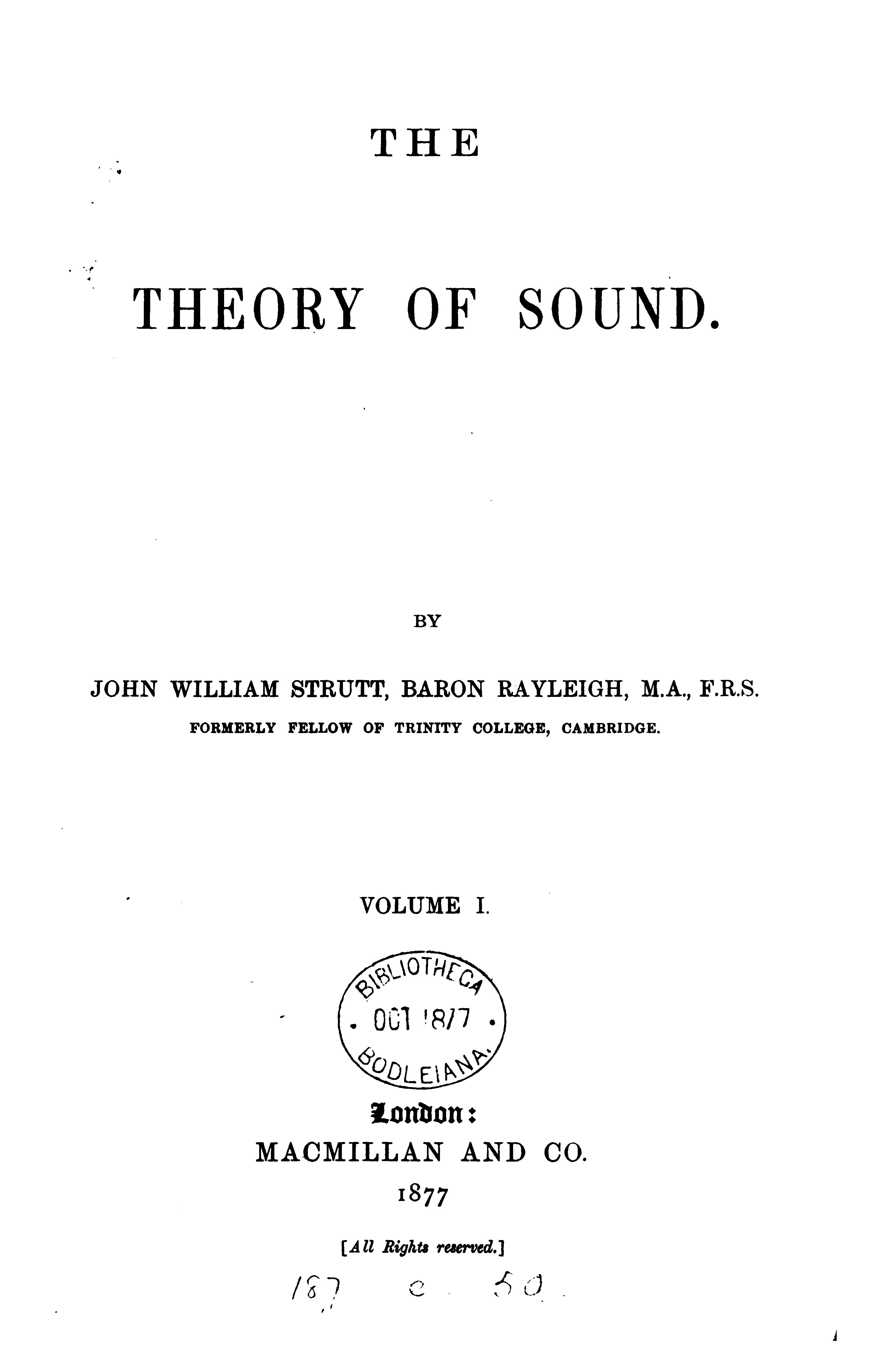
Rayleigh方程以及更多关于振动和声的内容可以这本非常经典的书中找到:
这两个方程的形式可以写成更加通用的形式:
$$ M y'' + k y = f(t, y, y') \tag{4} $$ODE初值问题的数值解
手工差分求解
对于 $y' = f(t, y, y')$ 这样的微分方程,考虑初值问题则需要给定初始条件$y(t_0) = y_0$和$y'(t_0) = y'_0$,然后求解在时间区间$[t_0, t_f]$上的解。
一清的同学很轻松地就能编一个Excel表格或Python脚本来求解这个方程。易知递推公式:
$$ y_{n+1} = y_n + h f(t_n, y_n, y'_n) \tag{5} $$如果结果不够好,调整步长$h$,直到满足精度要求。
这个方式的数值求解对于绝大部分工程问题来说就已经足够了。
我亲眼看到一清的同学用这个方法成功地求解过很多很多实际问题。
RK算法
如果学过数值方法,则会考虑使用Runge-Kutta(RK)方法。RK方法是一类常用的数值求解ODE的方法,特别是四阶RK方法(RK4)非常流行。实际上,RK4方法就是上面手工差分求解的一个更高精度的变种。
$$ y_{n+1} = y_n + \frac{h}{6} \left( k_1 + 2k_2 + 2k_3 + k_4 \right) \tag{6} $$其中,
$$ \begin{split} k_1 &= f(t_n, y_n, y'_n) \\ k_2 &= f(t_n + \frac{h}{2}, y_n + \frac{h}{2} k_1, y'_n + \frac{h}{2} k_1) \\ k_3 &= f(t_n + \frac{h}{2}, y_n + \frac{h}{2} k_2, y'_n + \frac{h}{2} k_2) \\ k_4 &= f(t_n + h, y_n + h k_3, y'_n + h k_3) \end{split} \tag{7} $$这两个方法都是显式数值求解方法,唯一的不同就只是差分精度。
matlab ODE求解器
Matlab提供了多种ODE求解器,适用于不同类型的ODE问题。根据ODE Solvers in MATLAB中ODE求解器的基本选择,第一个选择就是ode45,这是最常用的非刚性ODE求解器,基于Dormand-Prince方法(Runge-Kutta方法的一种)。适用于大多数非刚性问题,具有良好的精度和效率。
调用方式
我们可以通过help命令查看ode45的帮助信息:
 1 ode45  Solve non-stiff differential equations, medium order method.
 2  [TOUT,YOUT] = ode45(ODEFUN,TSPAN,Y0) integrates the system of
 3  differential equations y' = f(t,y) from time TSPAN(1) to TSPAN(end)
 4  with initial conditions Y0. Each row in the solution array YOUT
 5  corresponds to a time in the column vector TOUT.
 6    * ODEFUN is a function handle. For a scalar T and a vector Y,
 7    ODEFUN(T,Y) must return a column vector corresponding to f(t,y).
 8    * TSPAN is a two-element vector [T0 TFINAL] or a vector with
 9    several time points [T0 T1 ... TFINAL]. If you specify more than
10    two time points, ode45 returns interpolated solutions at the
11    requested times.
12    * YO is a column vector of initial conditions, one for each equation.
13
14  [TOUT,YOUT] = ode45(ODEFUN,TSPAN,Y0,OPTIONS) specifies integration
15  option values in the fields of a structure, OPTIONS. Create the
16  options structure with odeset.
17
18  [TOUT,YOUT,TE,YE,IE] = ode45(ODEFUN,TSPAN,Y0,OPTIONS) produces
19  additional outputs for events. An event occurs when a specified function
20  of T and Y is equal to zero. See ODE Event Location for details.
21
22  SOL = ode45(...) returns a solution structure instead of numeric
23  vectors. Use SOL as an input to DEVAL to evaluate the solution at
24  specific points. Use it as an input to ODEXTEND to extend the
25  integration interval.
26
27  ode45 can solve problems M(t,y)*y' = f(t,y) with mass matrix M that is
28  nonsingular. Use ODESET to set the 'Mass' property to a function handle
29  or the value of the mass matrix. ODE15S and ODE23T can solve problems
30  with singular mass matrices.
31
32  ODE23, ode45, ODE78, and ODE89 are all single-step solvers that use
33  explicit Runge-Kutta formulas of different orders to estimate the error
34  in each step.
35    * ode45 is for general use.
36    * ODE23 is useful for moderately stiff problems.
37    * ODE78 and ODE89 may be more efficient than ode45 on non-stiff problems
38    that are smooth except possibly for a few isolated discontinuities.
39    * ODE89 may be more efficient than ODE78 on very smooth problems, when
40    integrating over long time intervals, or when tolerances are tight.
41
42  Example
43      [t,y]=ode45(@vdp1,[0 20],[2 0]);
44      plot(t,y(:,1));
45    solves the system y' = vdp1(t,y), using the default relative error
46    tolerance 1e-3 and the default absolute tolerance of 1e-6 for each
47    component, and plots the first component of the solution.
48
49  Class support for inputs TSPAN, Y0, and the result of ODEFUN(T,Y):
50    float: double, single
51
52  See also ode23, ode78, ode89, ode113, ode15s, ode23s, ode23t, ode23tb,
53       ode15i, odeset, odeplot, odephas2, odephas3, odeprint, deval,
54       odeexamples, function_handle.
55
56  Documentation for ode45
57  Other uses of ode45
当然我们还可以通过doc ode45命令查看更详细的文档。
一般的调用方式:
1[t, y] = ode45(@odefun, tspan, y0);
或者
1sol = ode45(@odefun, tspan, y0);
这样就可以获得tspan时间区间内的ODE解。
当然,我们还可以不带输出参数,直接调用:
1ode45(@odefun, tspan, y0);
此时Matlab会自动绘制ODE解的图形。
ode45函数的输入参数中还可以增加一个options参数,用于设置ODE求解器的选项,例如相对误差和绝对误差等。
1options = odeset('RelTol',1e-6,'AbsTol',1e-9);
2[t, y] = ode45(@odefun, tspan, y0, options);
在options中,我们可以设置以下选项:
RelTol:相对误差容限,默认值为1e-3。AbsTol:绝对误差容限,默认值为1e-6。MaxStep:最大步长,默认值为0,表示不限制步长。InitialStep:初始步长,默认值为0,表示自动选择。Events:事件函数,用于检测ODE求解过程中的事件。
在options参数之后,还可以增加一个额外的自定义参数,这个参数会被同步传递给ODE函数odefun。
1[t, y] = ode45(@(t, y) odefun(t, y, param), tspan, y0);
这种构造临时函数额方式也可以写成:
1[t, y] = ode45(@odefun, tspan, y0, [], param);
被积函数
被积函数odefun需要满足以下要求:
- 至少接受两个输入参数:时间
t和状态变量y。 - 可以接受第三个参数自定义参数,在
ode45调用时传递。 - 返回一个列向量,表示ODE的右侧函数值。
- 可以是一个函数句柄或匿名函数。
1function dydt = odefun(t, y, param)
2  % 这里的param可以是一个自定义参数
3  dydt = zeros(2, 1); % 假设有两个变量
4  dydt(1) = y(2); % y1' = y2
5  dydt(2) = -param * y(1); % y2' = -param * y1
6end
Rayleigh方程的Matlab求解
odefun代码
首先,我们定义Rayleigh方程的ODE函数,这里把$\mu$作为一个参数传递给ODE函数:
1function dydt = rayleigh_ode(t, y, mu)
2% Rayleigh ODE function
3% dydt = rayleigh(t, y, mu)
4% t: time variable
5% y: state variable (y(1) = y, y(2) = dy/dt)
6dydt = zeros(2, 1);
7dydt(1) = y(2);
8dydt(2) = mu * (1 - (1/3) * y(2)^2) * y(2) - y(1);
9end
这里为了清晰,采取了标量形式的Rayleigh方程,对于更容易写成向量形式的微分方程组,可以直接采用恰当的matlab惯用表达方式。比如硬要拗姿势的话,上面的函数可以写成:
1function dydt = odefun(t, y, mu)
2dydt = [0, 1;...
3  -1, mu * (1 - (1/3) * y(2)^2)] * y(:);
4end
或者:
1odefun = @(t, y, mu)[0, 1;...
2 -1, mu * (1 - (1/3) * y(2)^2)] * y(:);
3
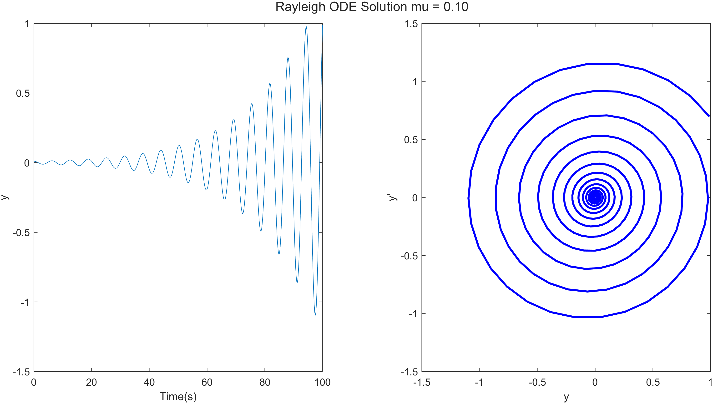
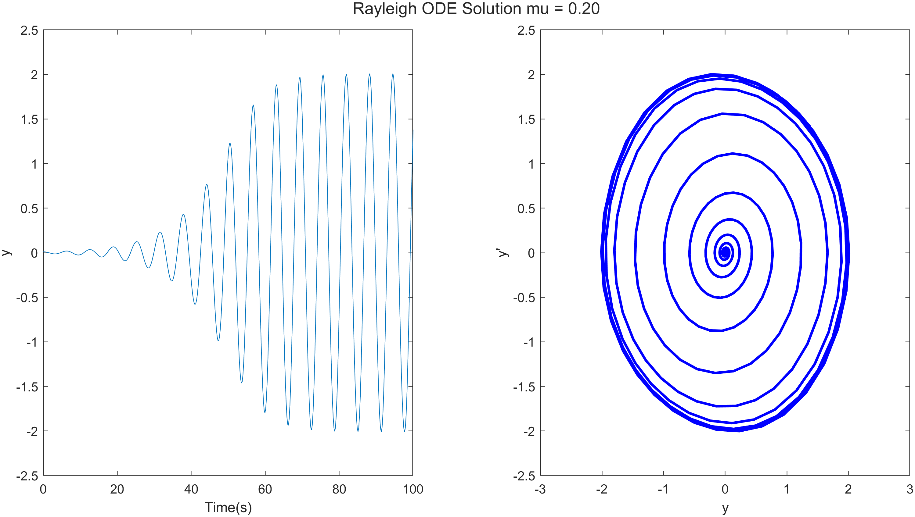
4ode45(odefun, [0 100], [0.1; 0], [], 0.1);
这样就会直接积分出结果并绘制y和y'的图像如下图:
的确是非常方便。
其它
我们对函数的参数进行了限制,并设置了默认值:
1arguments
2    mu (1,1) double {mustBeNumeric, mustBeFinite} = 0.4; % Default value for mu
3    show_fig (1,1) logical = false; % Default value for show_fig
4    y_1_0 (1,1) double {mustBeNumeric, mustBeFinite} = 0.001;
5end
arguments...end这个语法,功能还是非常强大的。
当然,我们还是整了点其它代码来得到更加漂亮的图。
1tl = tiledlayout(1,2);
2title(tl, sprintf('Rayleigh ODE Solution mu = %.2f', mu));
3
4nexttile
5plot(t, y(:, 1))
6xlabel('Time(s)')
7ylabel('y')
用tiledlayout来进行图形的简单排列。
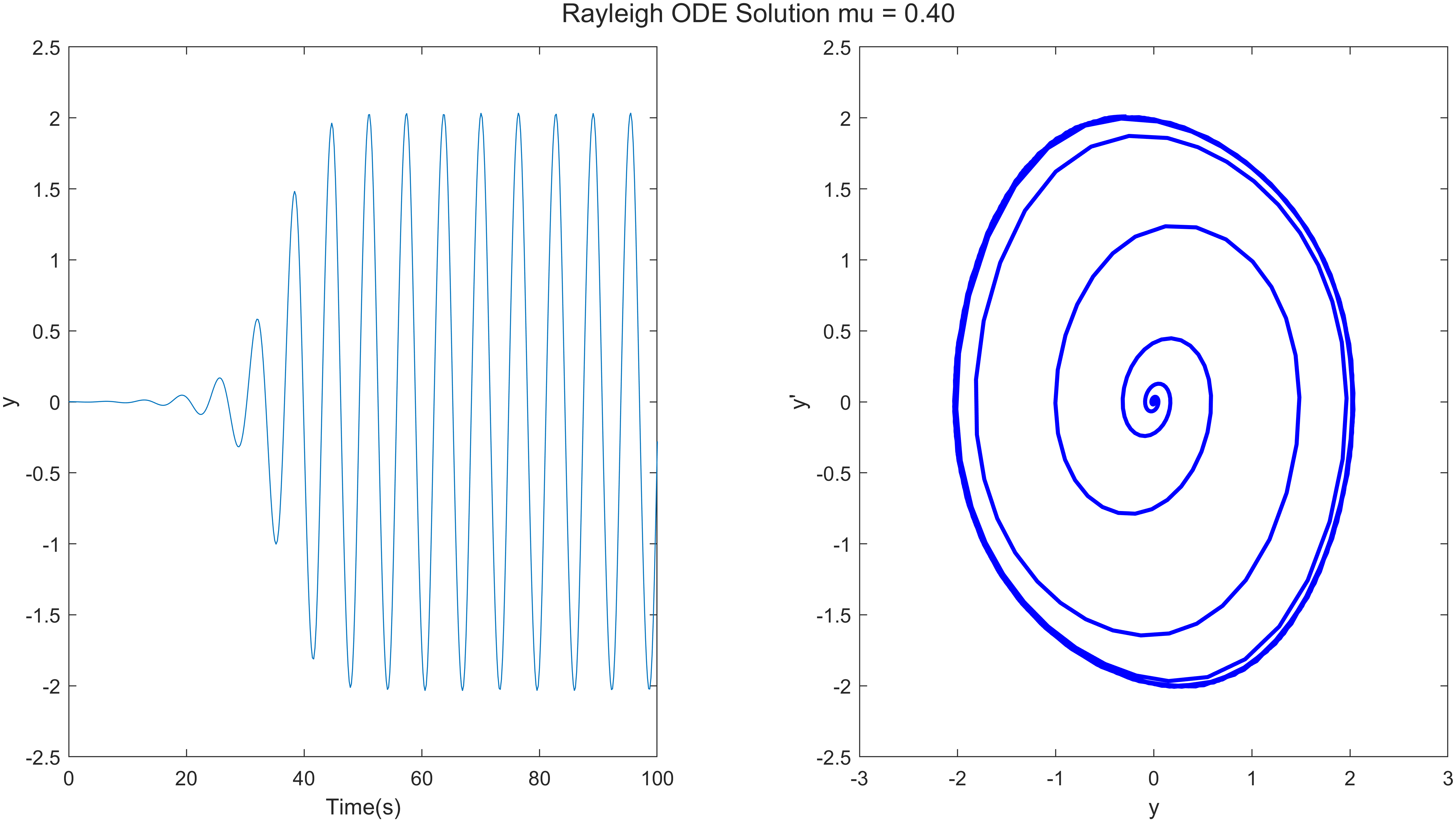
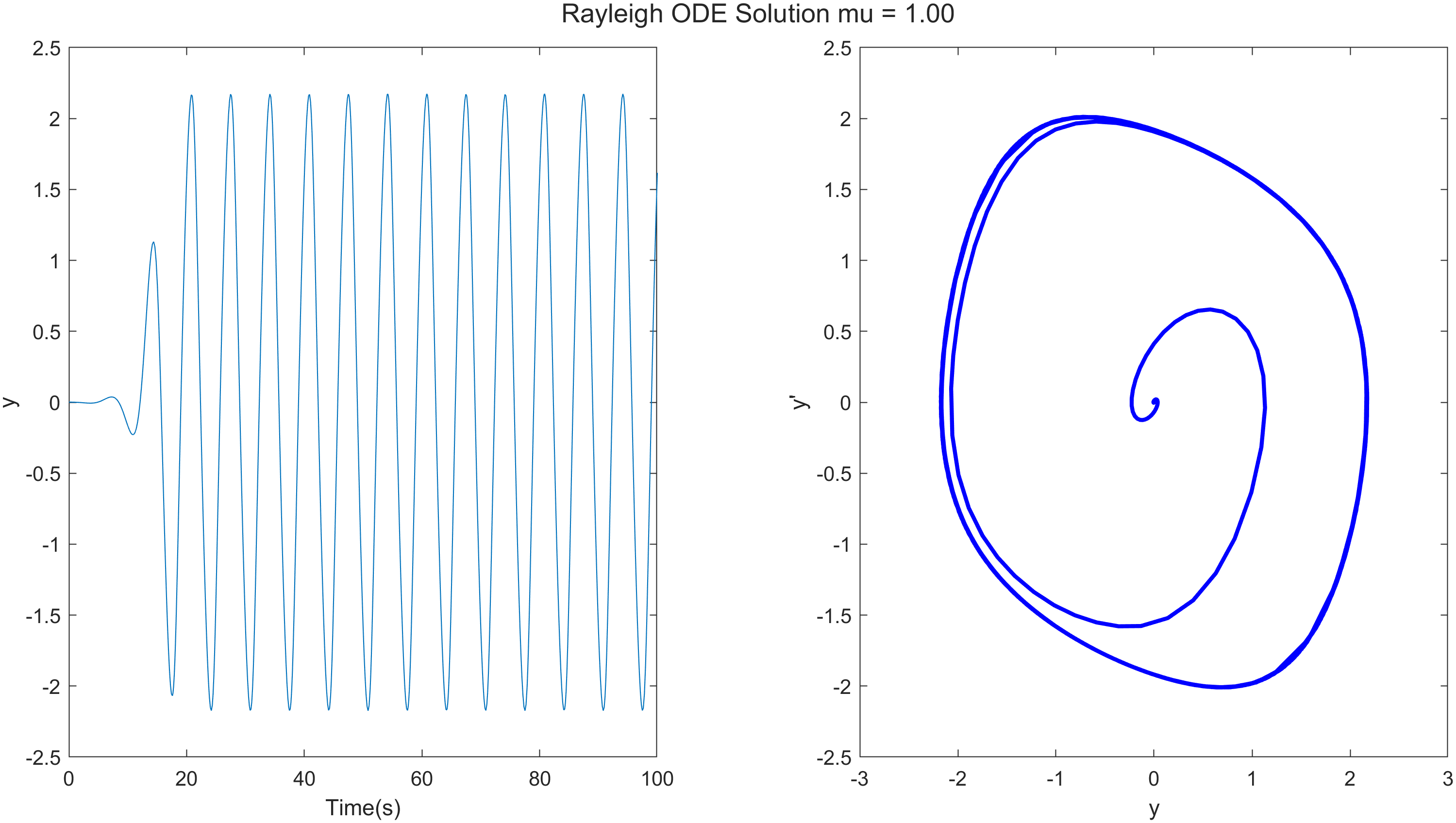
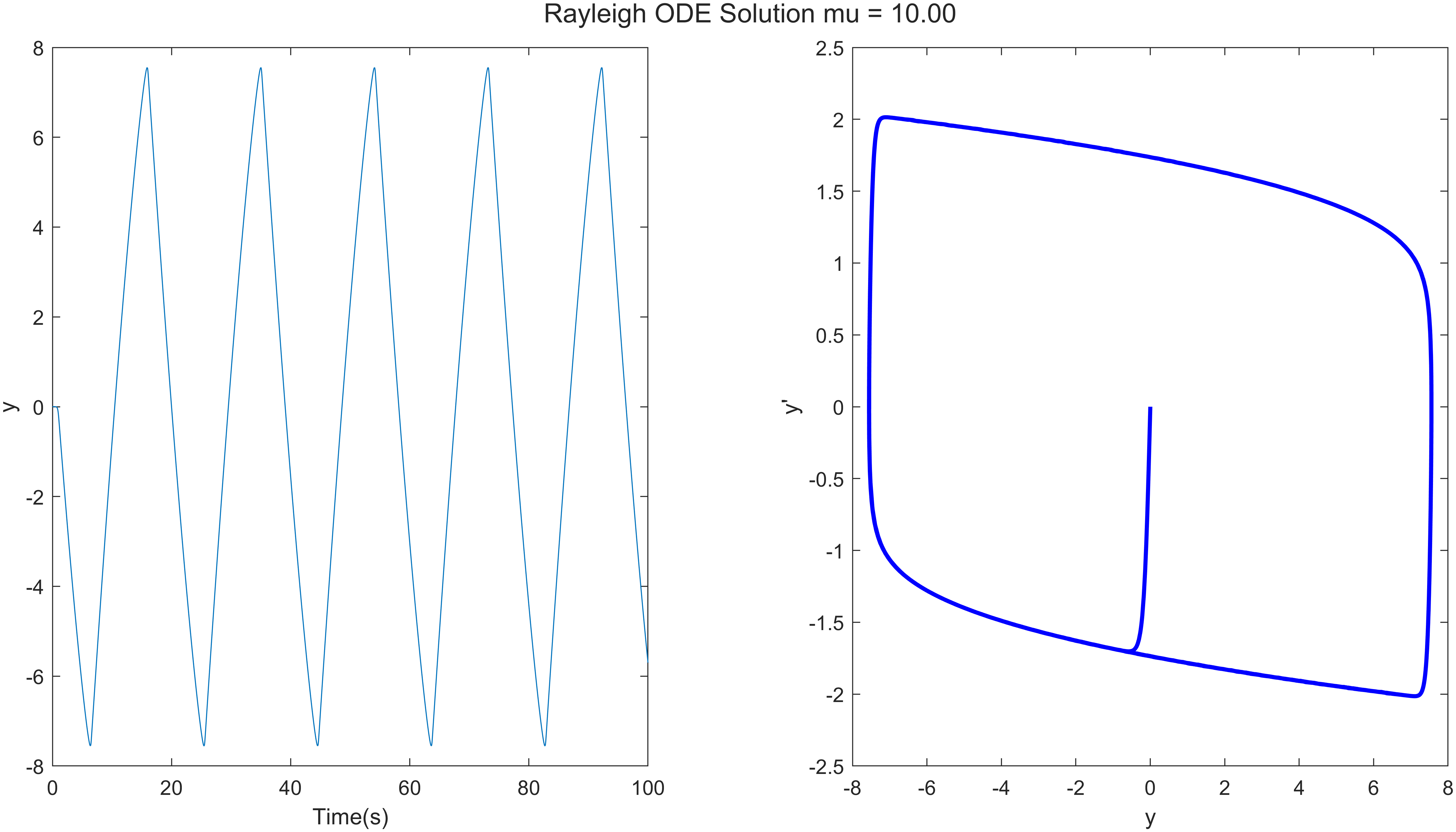
对参数进行研究是常规的,例如,比较不同$\mu$的结果。
完整的代码:
 1function rayleigh(mu, show_fig, y_1_0)
 2arguments
 3    mu (1,1) double {mustBeNumeric, mustBeFinite} = 0.4; % Default value for mu
 4    show_fig (1,1) logical = false; % Default value for show_fig
 5    y_1_0 (1,1) double {mustBeNumeric, mustBeFinite} = 0.001;
 6end
 7
 8y0 = [y_1_0; 0]; % Initial conditions: y(0) = 0, dy/dt(0) = 1
 9tspan = [0 100]; % Time span for the solution
10
11
12fig = figure('Units','inches', 'Position', [1, 1, 12, 6], 'Visible', false);
13
14% [t, y] = ode45(@(t, y) rayleigh_ode(t, y, mu), tspan, y0);
15[t, y] = ode45(@rayleigh_ode, tspan, y0, [], mu);
16
17tl = tiledlayout(1,2);
18title(tl, sprintf('Rayleigh ODE Solution mu = %.2f', mu));
19
20nexttile
21plot(t, y(:, 1))
22xlabel('Time(s)')
23ylabel('y')
24
25nexttile
26plot(y(:,1), y(:,2), 'b-', 'LineWidth', 2);
27xlabel('y')
28ylabel('y''')
29
30exportgraphics(tl, sprintf('rayleigh_solution_%.2f.png', mu), 'Resolution', 500);
31
32if show_fig
33    set(fig, 'Visible', 'on');
34else
35    close(fig); % Close the figure if not showing
36end
37end
38
39function dydt = rayleigh_ode(t, y, mu)
40% Rayleigh ODE function
41% dydt = rayleigh(t, y, mu)
42% t: time variable
43% y: state variable (y(1) = y, y(2) = dy/dt)
44dydt = zeros(2, 1);
45dydt(1) = y(2);
46dydt(2) = mu * (1 - (1/3) * y(2)^2) * y(2) - y(1);
47end
结论
简单的ode45,用默认值就能够获得很好的数值结果。
后面再来考虑增加事件来处理动力学的不同阶段。
或者再对簧片振动来做点有限元?
文章标签
|-->ode |-->Rayleigh |-->van der Pol |-->Rayleigh ODE |-->MATLAB ODE Solvers |-->MATLAB ODE Basics
- 本站总访问量:loading次
- 本站总访客数:loading人
- 可通过邮件联系作者:Email大福
- 也可以访问技术博客:大福是小强
- 也可以在知乎搞抽象:知乎-大福
- Comments, requests, and/or opinions go to: Github Repository