2024-10-28 |欢迎您，第位读者！|

Common_Plots_Matlab常见二维绘图

常用的二维绘图

常用绘图包括下面的种类：

• 线图， plot
• 柱图， bar
• 梯步图，stairstep
• 误差棒图，errorbar
• 极坐标图，polarplot
• 跟图，stem
• 散点图，scatter

这些命令都可以通过help xxx来查看基本的帮助，并通过doc xxx来查看详细的帮助，帮助中通常还有海量的例子来学习如何调用，并且在高版本的Matlab里面，还能打开相应的LiveScript，修改参数查看绘图结果。

详细介绍每个函数感觉必要性不大，还不如看一些通用的概念，能够更好应对实际应用中可能出现的状况。

这有一个小例子，可以展示出了极坐标之外的所有几种常规图形的绘制。可以通过按钮和菜单选择相应的函数，查看相应的图形。

代码文件下载：plotExample

这里把源文件内容也列在这里：

  1function f = common2DPlots
  2f = uifigure(Name='Common 2D Plots', Visible='off', WindowState='minimized');
  3movegui(f, 'center');
  4g = uigridlayout(f, [1, 1]);
  5ax = uiaxes(g, Visible='off');
  6ax.Layout.Row = 1;
  7ax.Layout.Column = 1;
  8
  9menu = uimenu(f, Text="Demos");
 10tb = uitoolbar(f);
 11
 12texts = {...
 13    "Line Plots", ...
 14    "Multiple Lines Plots", ...
 15    "Bar Plots", ...
 16    "Stairstep Plots", ...
 17    "Errorbar Plots", ...
 18    "Stem Plots", ...
 19    "Scatter Plots", ...
 20    "Scatter Colorbar Plots", ...
 21    };
 22fcns = {...
 23    @linePlotFcn, ...
 24    @multipleLinePlotFcn, ...
 25    @barPlot,...
 26    @stairStepPlot, ...
 27    @errorBarPlot, ...
 28    @stemPlot, ...
 29    @scatterPlot, ...
 30    @scatterColorPlot, ...
 31    };
 32n = numel(texts);
 33
 34for idx = 1:n
 35    fn = matlab.lang.makeValidName(texts{idx}) + ".png";
 36    
 37    if ~exist(fn, 'file')
 38        feval(fcns{idx}, ax);
 39        exportgraphics(ax, fn, Resolution=10);
 40    end
 41    
 42    cb = makeCallback(fcns{idx}, ax, texts{idx});
 43    
 44    uimenu(menu, Text=texts{idx}, ...
 45        MenuSelectedFcn=cb);
 46    uipushtool(tb, Tooltip=texts{idx}, ...
 47        Icon=fn, ...
 48        ClickedCallback=cb)
 49end
 50
 51uimenu(menu, Text="Quit", ...
 52    Accelerator="Q", ...
 53    Separator='on', ...
 54    MenuSelectedFcn=@(~, ~)close(f));
 55
 56
 57clearAll(ax);
 58
 59f.WindowState = "normal";
 60f.Visible = 'on';
 61
 62end
 63
 64function fh = makeCallback(func, ax_handle, textLabel)
 65    function retCb(~,  ~)
 66        clearAll(ax_handle);
 67        feval(func, ax_handle);
 68        ax_handle.Title.String = textLabel;
 69        ax_handle.Title.FontWeight = 'bold';
 70        ax_handle.Title.FontSize = 24;
 71        ax_handle.Visible = 'on';
 72    end
 73fh = @retCb;
 74end
 75
 76
 77function clearAll(ax_handle)
 78colorbar(ax_handle, 'off');
 79cla(ax_handle);
 80end
 81
 82function scatterPlot(ax_handle)
 83load patients Height Weight Systolic
 84scatter(ax_handle, Height,Weight)
 85xlabel(ax_handle,'Height')
 86ylabel(ax_handle,'Weight')
 87end
 88
 89function scatterColorPlot(ax_handle)
 90load patients Height Weight Systolic
 91scatter(ax_handle, Height,Weight, 20,Systolic)
 92xlabel(ax_handle,'Height')
 93ylabel(ax_handle,'Weight')
 94colorbar(ax_handle);
 95end
 96
 97
 98function stemPlot(ax_handle)
 99x = 0:0.1:4;
100y = sin(x.^2) .* exp(-x);
101stem(ax_handle, x, y);
102end
103
104function polarPlot(ax_handle)
105clearAll(ax_handle);
106theta = 0:0.01:2*pi;
107rho = abs(sin(2*theta) .* cos(2*theta));
108polarplot(ax_handle, theta, rho);
109end
110
111function errorBarPlot(ax_handle)
112x = -2:0.1:2;
113y = erf(x);
114eb = rand(size(x)) / 7;
115errorbar(ax_handle, x, y, eb);
116end
117
118
119function stairStepPlot(ax_handle)
120x = 0:0.25:10;
121y = sin(x);
122stairs(ax_handle, x, y);
123end
124
125function barPlot(ax_handle)
126x = -2.9:0.2:2.9;
127y = exp(-x .* x);
128bar(ax_handle, x, y);
129end
130
131
132function linePlotFcn(ax_handle)
133x = 0:0.05:5;
134y = sin(x.^2);
135plot(ax_handle, x, y);
136end
137
138function multipleLinePlotFcn(ax_handle)
139x = 0:0.05:5;
140y1 = sin(x.^2);
141y2 = cos(x.^2);
142plot(ax_handle, x, y1, x, y2);
143end

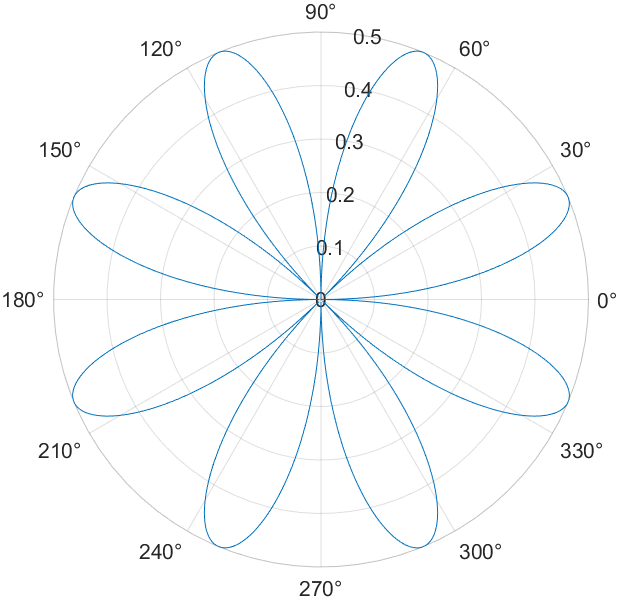
而极坐标图，可以通过polarplot函数来绘制。

1theta = 0:0.01:2*pi;
2rho = abs(sin(2*theta).*cos(2*theta));
3polarplot(theta,rho)

因为极坐标图对应的坐标是PolarAxes对象，跟上面这个小小的例子不太容易搞到一起，所以这里就不放在这个例子里面了。

图形窗口和坐标系

首先对于一个图形，最基本的两个概念就是：

1. 图形窗口
2. 坐标系

这两个前者是实体的画布，后者是概念的画布。实际的图线，都要画在图形窗口的像素上；而图线对应点的坐标数据，则映射在坐标系中。

在实际的对象层次结构中，Matlab中图形窗口对象Figre有一个属性Childeren ，是一个数组，中间有若干坐标系；而代表坐标系的Axes ，也有一个属性Children ，也是一个数组，里面放着若干图形对象。

graph TD
G[groot] -->|Children| A[Figure] -->|Children| B[Axes]
B -->|Children| C[Line]

对下面这个例子可以看到相应的关系。

 1x = 0:0.1:2*pi;
 2y = sin(x);
 3
 4% 
 5f = gcf;  % 如果当前没有活动的窗口句柄则自动调用`gcf`创建一个图形窗口
 6a = gca;
 7
 8% l = plot(x, y); 自动调用`gca`获得默认的笛卡尔坐标系
 9l = plot(a, x, y);
10
11a1 = sprintf('图线对象是否在坐标系的Children中：       %d\n', ismember(l, a.Children));
12a2 = sprintf('坐标系对象是否在图形窗口的Children中：%d\n', ismember(a, f.Children));
13
14title([a1 a2])

​

​
​

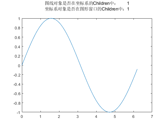
这里，我们用gcf来得到一个图窗对象，用gca来得到一个默认的笛卡尔坐标系。实际上，我们调用上述绘图函数的时候，可以把第一个参数设置为一个坐标系对象，如果省略这个参数，Matlab会自动调用gca来作为坐标系对象，并把绘图函数返回的图形对象加入（append）到对应坐标系的Children属性中。

gcf和gca两个函数都是称为lazy的函数，如果最近有一个句柄可见（Figure和Axes对象的HandleVisibility属性）的对象，就返回，如果没有，那就新建一个。这个过程是逐级向上的。例如，我们在没有图形窗口的情况下调用gca，就会触发如下的流程。

1. 通过groot的Children逐步找下来，看是否有一个句柄可见的Axes对象
2. 没有的话需要新建一个Axes 3. gcf一个y图窗Figure对象 4. 试图从groot的Children逐步找下来，没有找到一个句柄可见的Figure对象 5. 新建一个Figure对象，添加到groot的Children中 6. 把新建的坐标系添加到图窗的Children中
3. 返回坐标系对象

我们可以自己在groot开始，翻找Children构成的树结构，也可以调用函数findobj来看看组合条件查看对象，当然直接调用不带任何参数返回所有的图形对象。

1help findobj

 findobj - 查找具有特定属性的图形对象
    此 MATLAB 函数 返回图形根对象及其所有后代。

    语法
      h = findobj
      h = findobj(prop,value)
      h = findobj('-not',prop,value)
      h = findobj(prop1,value1,oper,prop2,value2)
      h = findobj('-regexp',prop,expr)
      h = findobj('-property',prop)
      h = findobj(prop1,value1,...,propN,valueN)
      h = findobj(objhandles,___)
      h = findobj(objhandles,'-depth',d,___)
      h = findobj(objhandles,'flat',___)

    输入参数
      prop - 属性名称
        字符向量 | 字符串标量
      value - 属性值
        标量 | 数组
      oper - 逻辑运算符
        '-and' (默认值) | '-or' | '-xor'
      expr - 正则表达式
        字符串数组 | 字符向量 | 字符向量元胞数组
      objhandles - 要从中搜索的对象
        图形对象数组
      d - 搜索深度
        非负整数

    示例
      openExample('graphics/ReturnAllGraphicsObjectsExample')
      openExample('graphics/FindAllLineObjectsExample')
      openExample('graphics/FindObjectsWithSpecifiedPropertyValuesExample')
      openExample('graphics/FindObjectsWithoutSpecificPropertyValuesExample')
      openExample('graphics/FindObjectsUsingRegularExpressionExample')
      openExample('graphics/FindAllObjectsWithSpecifiedPropertyExample')
      openExample('graphics/FindAllLineObjectsInCurrentAxesExample')
      openExample('graphics/ReturnAllObjectsInCurrentFigureExample')
      openExample('graphics/RestrictSearchDepthExample')

    另请参阅 copyobj, findall, findobj, gcf, gca, gcbo, gco, get, regexp,
      set, groot

    已在 R2006a 之前的 MATLAB 中引入
    findobj 的文档
       doc findobj

    findobj 的其他用法

       handle/findobj    qrandstream/findobj

这个函数的功能非常强大，可以通过各种条件来查找对象，例如查找所有的Line对象，查找所有的Axes对象，查找所有的Figure对象等等。还能通过设置逻辑条件，正则表达式等等来查找对象。 ​

图像窗口

图像窗口的创建，可以用下面的函数来实现：

• gcf
• figure
• figure('Name', 'xxx')

这些函数返回一个Figure对象，可以通过get和set来查看和修改属性。属性的修改，也能够用过f.Name = 'xxx'这样的方式来实现。此外，调用操作坐标系的函数以及绘图函数（自动调用坐标系创建），也会自动修改图形窗口的属性。

1f = gcf;
2
3get(f)

得到所有属性的列表如下，可以自己查看。

                 Alphamap: [0 0.0159 0.0317 0.0476 0.0635 0.0794 0.0952 0.1111 0.1270 0.1429 0.1587 0.1746 0.1905 ... ] (1x64 double)
             BeingDeleted: off
               BusyAction: 'queue'
            ButtonDownFcn: ''
                 Children: [0x0 GraphicsPlaceholder]
                 Clipping: on
          CloseRequestFcn: 'closereq'
                    Color: [0.9400 0.9400 0.9400]
                 Colormap: [256x3 double]
              ContextMenu: [0x0 GraphicsPlaceholder]
                CreateFcn: ''
              CurrentAxes: [0x0 GraphicsPlaceholder]
         CurrentCharacter: ''
            CurrentObject: [0x0 GraphicsPlaceholder]
             CurrentPoint: [0 0]
                DeleteFcn: ''
             DockControls: on
                 FileName: ''
        GraphicsSmoothing: on
         HandleVisibility: 'on'
                     Icon: ''
            InnerPosition: [680 458 560 420]
            IntegerHandle: on
            Interruptible: on
           InvertHardcopy: on
              KeyPressFcn: ''
            KeyReleaseFcn: ''
                  MenuBar: 'figure'
                     Name: ''
                 NextPlot: 'add'
                   Number: 1
              NumberTitle: on
            OuterPosition: [676 454 568 454]
         PaperOrientation: 'portrait'
            PaperPosition: [0 0 5.8333 4.3750]
        PaperPositionMode: 'manual'
                PaperSize: [8.2677 11.6929]
                PaperType: 'A4'
               PaperUnits: 'inches'
                   Parent: [1x1 Root]
                  Pointer: 'arrow'
        PointerShapeCData: [16x16 double]
      PointerShapeHotSpot: [1 1]
                 Position: [680 458 560 420]
                 Renderer: 'opengl'
             RendererMode: 'auto'
                   Resize: on
               Scrollable: off
            SelectionType: 'normal'
           SizeChangedFcn: ''
                      Tag: ''
                  ToolBar: 'auto'
                     Type: 'figure'
                    Units: 'pixels'
                 UserData: []
                  Visible: off
      WindowButtonDownFcn: ''
    WindowButtonMotionFcn: ''
        WindowButtonUpFcn: ''
        WindowKeyPressFcn: ''
      WindowKeyReleaseFcn: ''
     WindowScrollWheelFcn: ''
              WindowState: 'normal'
              WindowStyle: 'normal'

​ 同时，可以通过help来查看这个函数的帮助。

1help figure

 figure - 创建图窗窗口
    此 MATLAB 函数 使用默认属性值创建一个新的图窗窗口。生成的图窗为当前图窗。

    语法
      figure
      figure(Name,Value)
      f = figure(___)

      figure(f)
      figure(n)

    输入参数
      f - 目标图窗
        Figure 对象
      n - 目标图窗编号
        整数标量值

    名称-值参数
      Name - 名称
        '' (默认值) | 字符向量 | 字符串标量
      Color - 背景色
        RGB 三元组 | 十六进制颜色代码 | 'r' | 'g' | 'b'
      Position - 可绘制区域的位置和大小
        [left bottom width height]
      Units - 测量单位
        'pixels' (默认值) | 'normalized' | 'inches' | 'centimeters' |
        'points' | 'characters'

    另请参阅 axes, gcf, gca, clf, cla, shg, Figure 属性

    已在 R2006a 之前的 MATLAB 中引入
    figure 的文档
       doc figure

​
​

坐标系对象

同样，坐标系对象的创建，可以用下面的函数来实现：

• gca
• axes

这些函数返回一个Axes对象，可以通过get和set来查看和修改属性。属性的修改，也能够用过a.XLim = [0, 1]这样的方式来实现。此外，调用绘图函数，也会自动修改坐标系的属性。

1a = gca;
2
3get(a)

                        ALim: [0 1]
                    ALimMode: 'auto'
                  AlphaScale: 'linear'
                    Alphamap: [0 0.0159 0.0317 0.0476 0.0635 0.0794 0.0952 0.1111 0.1270 0.1429 0.1587 0.1746 0.1905 ... ] (1x64 double)
           AmbientLightColor: [1 1 1]
                BeingDeleted: off
                         Box: off
                    BoxStyle: 'back'
                  BusyAction: 'queue'
               ButtonDownFcn: ''
                        CLim: [0 1]
                    CLimMode: 'auto'
              CameraPosition: [0.5000 0.5000 9.1603]
          CameraPositionMode: 'auto'
                CameraTarget: [0.5000 0.5000 0.5000]
            CameraTargetMode: 'auto'
              CameraUpVector: [0 1 0]
          CameraUpVectorMode: 'auto'
             CameraViewAngle: 6.6086
         CameraViewAngleMode: 'auto'
                    Children: [0x0 GraphicsPlaceholder]
                    Clipping: on
               ClippingStyle: '3dbox'
                       Color: [1 1 1]
                  ColorOrder: [7x3 double]
             ColorOrderIndex: 1
                  ColorScale: 'linear'
                    Colormap: [256x3 double]
                 ContextMenu: [0x0 GraphicsPlaceholder]
                   CreateFcn: ''
                CurrentPoint: [2x3 double]
             DataAspectRatio: [1 1 1]
         DataAspectRatioMode: 'auto'
                   DeleteFcn: ''
                   FontAngle: 'normal'
                    FontName: 'Helvetica'
                    FontSize: 10
                FontSizeMode: 'auto'
               FontSmoothing: on
                   FontUnits: 'points'
                  FontWeight: 'normal'
                   GridAlpha: 0.1500
               GridAlphaMode: 'auto'
                   GridColor: [0.1500 0.1500 0.1500]
               GridColorMode: 'auto'
               GridLineStyle: '-'
               GridLineWidth: 0.5000
           GridLineWidthMode: 'auto'
            HandleVisibility: 'on'
                     HitTest: on
               InnerPosition: [0.1300 0.1100 0.7750 0.8150]
          InteractionOptions: [1x1 matlab.graphics.interaction.interactionoptions.InteractionOptions]
                Interactions: [1x1 matlab.graphics.interaction.interface.DefaultAxesInteractionSet]
               Interruptible: on
     LabelFontSizeMultiplier: 1.1000
                       Layer: 'bottom'
                      Layout: [0x0 matlab.ui.layout.LayoutOptions]
                      Legend: [0x0 GraphicsPlaceholder]
      LineStyleCyclingMethod: 'aftercolor'
              LineStyleOrder: '-'
         LineStyleOrderIndex: 1
                   LineWidth: 0.5000
              MinorGridAlpha: 0.2500
          MinorGridAlphaMode: 'auto'
              MinorGridColor: [0.1000 0.1000 0.1000]
          MinorGridColorMode: 'auto'
          MinorGridLineStyle: ':'
          MinorGridLineWidth: 0.5000
      MinorGridLineWidthMode: 'auto'
                    NextPlot: 'replace'
             NextSeriesIndex: 1
               OuterPosition: [0 0 1 1]
                      Parent: [1x1 Figure]
               PickableParts: 'visible'
          PlotBoxAspectRatio: [1 0.7903 0.7903]
      PlotBoxAspectRatioMode: 'auto'
                    Position: [0.1300 0.1100 0.7750 0.8150]
          PositionConstraint: 'outerposition'
                  Projection: 'orthographic'
                    Selected: off
          SelectionHighlight: on
                  SortMethod: 'childorder'
                    Subtitle: [1x1 Text]
          SubtitleFontWeight: 'normal'
                         Tag: ''
                     TickDir: 'in'
                 TickDirMode: 'auto'
        TickLabelInterpreter: 'tex'
                  TickLength: [0.0100 0.0250]
                  TightInset: [0.0435 0.0532 0.0170 0.0202]
                       Title: [1x1 Text]
     TitleFontSizeMultiplier: 1.1000
             TitleFontWeight: 'normal'
    TitleHorizontalAlignment: 'center'
                     Toolbar: [1x1 AxesToolbar]
                        Type: 'axes'
                       Units: 'normalized'
                    UserData: []
                        View: [0 90]
                     Visible: on
                       XAxis: [1x1 NumericRuler]
               XAxisLocation: 'bottom'
                      XColor: [0.1500 0.1500 0.1500]
                  XColorMode: 'auto'
                        XDir: 'normal'
                       XGrid: off
                      XLabel: [1x1 Text]
                        XLim: [0 1]
                    XLimMode: 'auto'
                XLimitMethod: 'tickaligned'
                  XMinorGrid: off
                  XMinorTick: off
                      XScale: 'linear'
                       XTick: [0 0.1000 0.2000 0.3000 0.4000 0.5000 0.6000 0.7000 0.8000 0.9000 1]
                  XTickLabel: {11x1 cell}
              XTickLabelMode: 'auto'
          XTickLabelRotation: 0
      XTickLabelRotationMode: 'auto'
                   XTickMode: 'auto'
                       YAxis: [1x1 NumericRuler]
               YAxisLocation: 'left'
                      YColor: [0.1500 0.1500 0.1500]
                  YColorMode: 'auto'
                        YDir: 'normal'
                       YGrid: off
                      YLabel: [1x1 Text]
                        YLim: [0 1]
                    YLimMode: 'auto'
                YLimitMethod: 'tickaligned'
                  YMinorGrid: off
                  YMinorTick: off
                      YScale: 'linear'
                       YTick: [0 0.1000 0.2000 0.3000 0.4000 0.5000 0.6000 0.7000 0.8000 0.9000 1]
                  YTickLabel: {11x1 cell}
              YTickLabelMode: 'auto'
          YTickLabelRotation: 0
      YTickLabelRotationMode: 'auto'
                   YTickMode: 'auto'
                       ZAxis: [1x1 NumericRuler]
                      ZColor: [0.1500 0.1500 0.1500]
                  ZColorMode: 'auto'
                        ZDir: 'normal'
                       ZGrid: off
                      ZLabel: [1x1 Text]
                        ZLim: [0 1]
                    ZLimMode: 'auto'
                ZLimitMethod: 'tickaligned'
                  ZMinorGrid: off
                  ZMinorTick: off
                      ZScale: 'linear'
                       ZTick: [0 0.5000 1]
                  ZTickLabel: ''
              ZTickLabelMode: 'auto'
          ZTickLabelRotation: 0
      ZTickLabelRotationMode: 'auto'
                   ZTickMode: 'auto'

​
​默认创建的笛卡尔坐标系，两个坐标轴的范围都是[0, 1]，可以通过a.XLim和a.YLim来查看和修改。

​
​

1help axes

 axes - 创建笛卡尔坐标区
    此 MATLAB 函数 在当前图窗中创建默认的笛卡尔坐标区，并将其设置为当前坐标区。通常情况
    下，您不需要在绘图之前创建坐标区，因为如果不存在坐标区，图形函数会在绘图时自动创建坐标
    区。

    语法
      axes
      axes(Name,Value)
      axes(parent,Name,Value)
      ax = axes(___)

      axes(cax)

    输入参数
      parent - 父容器
        Figure 对象 | Panel 对象 | Tab 对象 | TiledChartLayout 对象 |
        GridLayout 对象
      cax - 要设置为当前坐标区的坐标区
        Axes 对象 | PolarAxes 对象 | GeographicAxes 对象 | 独立可视化

    名称-值参数
      Position - 大小和位置，不包括标签边距
        [0.1300 0.1100 0.7750 0.8150] (默认值) | 四元素向量
      OuterPosition - 大小和位置，包括标签和边距
        [0 0 1 1] (默认值) | 四元素向量
      Units - 位置单位
        "normalized" (默认值) | "inches" | "centimeters" | "points" |
        "pixels" | "characters"

    示例
      openExample('graphics/DefineMultipleAxesInFigureWindowExample')
      openExample('graphics/MakeSpecificAxesTheCurrentAxesExample')
      openExample('graphics/CreateAxesInUITabsExample')

    另请参阅 Axes 属性, axis, cla, gca, figure, clf, tiledlayout, nexttile,
      polaraxes

    已在 R2006a 之前的 MATLAB 中引入
    axes 的文档
       doc axes

对于Axes所有属性和设置的例子，文档同样列写得非常齐全。​
​
​

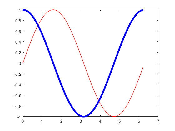
一个坐标系绘制多个图形

当我们调用plot函数时，可以直接提供多组数据，此时，Matlab会自动绘制多个图形，每个图形对应一组数据。返回的也是对应的图形对象的句柄。

可以通过对句柄的操作，来修改图形的属性，例如颜色，线型，线宽等等。

 1x = 0:0.1:2*pi;
 2y1 = sin(x);
 3y2 = cos(x);
 4
 5h = plot(x, y1, x, y2);
 6
 7h(1).Color = 'r';
 8h(2).Color = 'b';
 9
10h(1).LineWidth = 1;
11h(2).LineWidth = 4;

​
​

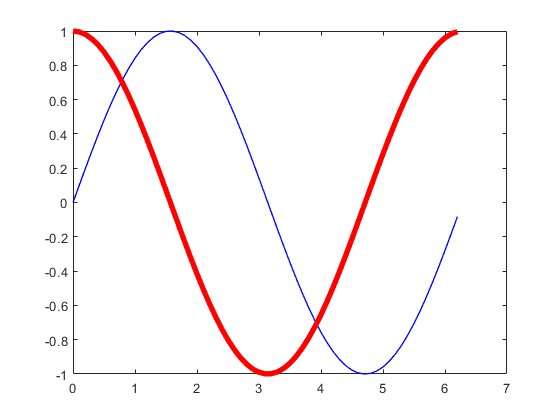
另外，我们也能通过hold('off')和hold('on')来控制是否保留原有的图形，这样也可以实现在一个坐标系中绘制多个图形。

绘制完毕图像，或者导入通过savefig保存的图像之后，还能通过findobj来查找图形对象，然后对其进行操作。

 1x = 0:0.1:2*pi;
 2y1 = sin(x);
 3y2 = cos(x);
 4
 5plot(x, y1)
 6hold('on');
 7
 8plot(x, y2);
 9
10
11% savefig('test.fig')
12% close('all')
13
14% openfig('test.fig')
15
16h = findobj(gca, 'Type', 'line');
17
18h(1).Color = 'r';
19h(2).Color = 'b';
20
21h(1).LineWidth = 4;
22h(2).LineWidth = 1;

​

​
​

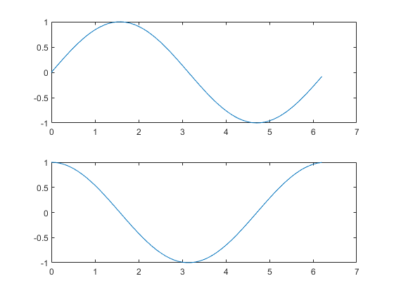
多坐标系绘图

把多个坐标系放在一个图形中，在发表论文的过程中是很常规的操作。以前Matlab采用的是subplot函数，现在推荐使用tiledlayout和nexttile函数。

 1% subplot example
 2
 3f = figure;
 4
 5a1 = subplot(2, 1, 1);
 6x = 0:0.1:2*pi;
 7y = sin(x);
 8plot(a1, x, y);
 9
10a2 = subplot(2, 1, 2);
11y = cos(x);
12plot(a2, x, y);

​

​
​

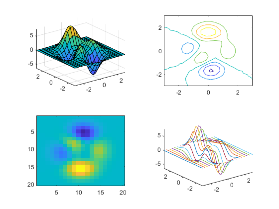
用新的工具，可以更加方便的控制坐标系的位置和大小，以及坐标系之间的间距。这个工具的使用方法，可以参考doc tiledlayout和doc nexttile。

下面是一个非常简单的例子，展示了如何使用这个工具。

 1tiledlayout(2,2);
 2[X,Y,Z] = peaks(20);
 3
 4% Tile 1
 5nexttile
 6surf(X,Y,Z)
 7
 8% Tile 2
 9nexttile
10contour(X,Y,Z)
11
12% Tile 3
13nexttile
14imagesc(Z)
15
16% Tile 4
17nexttile
18plot3(X,Y,Z)

可以看到，每个Axes都是一个独立可以进行二维乃至三维绘图的区域。从这一点上来看，Matlab的绘图功能的确比Python的matplotlib要强不少。

​
​

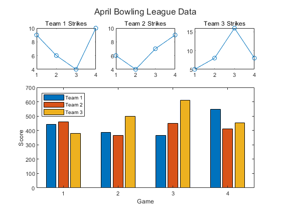
更加复杂的布局方式，还可以通过，nexttile([2, 2])这样的方式来实现多行多列的子图。

 1scores = [444 460 380 
 2          387 366 500 
 3          365 451 611 
 4          548 412 452];
 5
 6strikes = [9  6  5  
 7           6  4  8 
 8           4  7  16  
 9           10 9  8];
10     
11t = tiledlayout('flow');
12
13% Team 1
14nexttile
15plot([1 2 3 4],strikes(:,1),'-o')
16title('Team 1 Strikes')
17
18% Team 2
19nexttile
20plot([1 2 3 4],strikes(:,2),'-o')
21title('Team 2 Strikes')
22
23% Team 3
24nexttile
25plot([1 2 3 4],strikes(:,3),'-o')
26title('Team 3 Strikes')
27
28% 设置两行三列的子图
29nexttile([2 3]);
30bar([1 2 3 4],scores)
31legend('Team 1','Team 2','Team 3','Location','northwest')
32
33% Configure ticks and axis labels
34xticks([1 2 3 4])
35xlabel('Game')
36ylabel('Score')
37
38% Add layout title
39title(t,'April Bowling League Data')

tiledlayout可以通过参数设置横向、纵向、流式布局等等，具体的参数可以参考doc tiledlayout。最后那个nexttile([2 3])的参数，可以设置子图的大小，这个参数是一个二维数组，第一个元素是行数，第二个元素是列数。

​
​

同样，我们也能通过help和doc来查看这些函数的帮助。

• doc tiledlayout
• doc nexttile
• doc tilenum
• doc tilerowcol

这四个函数全部需要R2022b以后的版本。

实际上，这个话题值得单独开一个帖子来讨论。