2024-12-31 |欢迎您，第位读者！|

008 Kotlin 中干点正经活：搜索一维函数最小值

正经干活

其实，我还是经常用Kotlin干正经事情的。以前也用一些Java，现在用上Kotlin之后，Java顿时就不香了。特别是用了amper之后，项目的干净程度又上升一个台阶。不用再写什么build.gradle.kts了，直接用amper的DSL就可以了。

问题

这一次，来展示一下用解决一个简单的问题：搜索一维函数的最小值。

目标函数

就随便写一个函数：

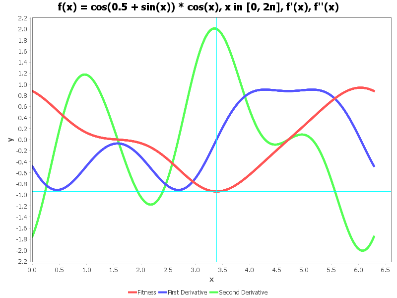
$$ f(x) = \cos (0.5 + \sin x) \cos x, x \in [0, 2\pi] $$

实现为Kotlin代码：

1import kotlin.math.cos
2import kotlin.math.sin
3
4fun fitness(d: Double): Double {
5    return cos(0.5 + sin(d)) * cos(d)
6}

极小值条件

这个函数的最小值从图形上很容易看到，实在是太简单了。并且，从数学中我们可以得到最小值所在位置 $x^\*$ 满足：

$$ \begin{cases} f'(x^\*) = 0 \\\\ f''(x^\*) > 0 \end{cases} $$

从上面的图中可以看到，极值点有两个，最小值的点有一个。按照导数和二次导数的关系，也能通过网格搜索找到最小值的位置。

网格生成

要实现网格搜索，首先我们定义一个生成线性网络的函数，给定区间和点数，生成一个线性的网络，表达为Array<Double>。

1fun linspace(start: Double, stop: Double, num: Int): Array<Double> {
2    val step = (stop - start) / (num - 1)
3    return Array(num) { i -> start + i * step }
4}

这个要这么设计而不是通过步长来产生主要是为了偷懒，如果设置步长的话，就必须处理步长不能整除的情况，要搞半天。反过来就简单多了。

导数计算

当然，要按照前面的极小值条件来找到最小值，就需要计算导数。这里我们用数值方法来计算导数，这样就不用去解析求导了。

1fun derive(f: (Double) -> Double, x: Double, h: Double = 1e-6): Double {
2    return (8 * f(x + h) + f(x - 2 * h) - (f(x + 2 * h) + 8 * f(x - h))) / (12.0 * h)
3}
4
5
6fun derive2(f: (Double) -> Double, x: Double, h: Double = 1e-6): Double {
7    return (16 * (f(x + h) + f(x - h)) - (30 * f(x) + f(x + 2 * h) + f(x - 2 * h))) / (12.0 * h * h)
8}

我们用了一个高精度方法来计算导数和二阶导数，这样步长的选择就可以稍微简单一点。高阶的方法有个代价，就是需要计算更多的目标函数，这里需要计算9次才能得到导数和二阶导数。

有了这两个函数，就想着实现一个设定步长，一次性表达 $x, f(x), f'(x), f''(x)$ 的方式，在Kotlin这样的高糖语言中，都不是事。

 1data class FunctionPointAndDerivatives(
 2    val point: Double, val fitness: Double, val firstDerivative: Double, val secondDerivative: Double
 3) {
 4    companion object {
 5        private var _h = 1e-6
 6        var h: Double
 7            get() = _h
 8            set(value) {
 9                _h = value
10            }
11
12        fun of(x: Double, f: (Double) -> Double = { it }): FunctionPointAndDerivatives {
13            return FunctionPointAndDerivatives(x, f(x), derive(f, x, h), derive2(f, x, h))
14        }
15    }
16}

这个函数有两个好玩的，一个就是采用了data class；另外一个就是companion object，这个是Kotlin的一个特性，可以在类中定义一个伴生对象，这个对象的方法和属性可以直接通过类名访问，就像Java中的静态方法一样。

一般而言，我们就可以这样来调用：

1FunctionPointAndDerivatives.apply { h = 0.01}.of(0.0){x -> cos(0.5 + sin(x)) * cos(x)}

这样的调用方式，就相当完美了。

我还很无聊写了几个测试。

 1import kotlin.test.Test
 2import kotlin.test.assertEquals
 3import kotlin.test.assertTrue
 4import kotlin.math.cos
 5import kotlin.math.sin
 6
 7class DeriveTest {
 8    val epsilon = 1e-9
 9    val hD = 1e-3
10
11    @Test
12    fun testSimpleDerive() {
13        fun f(x: Double): Double {
14            return x * x
15        }
16
17        val x = 2.0
18        val dfs = FunctionPointAndDerivatives.apply { h = hD }.of(x, ::f)
19        assertEquals(x, dfs.point, epsilon)
20        assertEquals(x * x, dfs.fitness, epsilon)
21        assertEquals(2.0 * x, dfs.firstDerivative, epsilon)
22        assertEquals(2.0, dfs.secondDerivative, epsilon)
23    }
24
25    @Test
26    fun testSinDerive() {
27        val theta = 0.5
28        val dfs = FunctionPointAndDerivatives.apply { h = hD }.of(theta) {
29            sin(it)
30        }
31
32        assertEquals(theta, dfs.point, epsilon)
33        assertEquals(sin(theta), dfs.fitness, epsilon)
34        assertEquals(cos(theta), dfs.firstDerivative, epsilon)
35        assertEquals(-sin(theta), dfs.secondDerivative, epsilon)
36    }
37
38    @Test
39    fun testCosDerive() {
40        val theta = 0.5
41        val dfs = FunctionPointAndDerivatives.apply { h = hD }.of(theta) {
42            cos(it)
43        }
44
45        assertEquals(theta, dfs.point, epsilon)
46        assertEquals(cos(theta), dfs.fitness, epsilon)
47        assertEquals(-sin(theta), dfs.firstDerivative, epsilon)
48        assertEquals(-cos(theta), dfs.secondDerivative, epsilon)
49    }
50
51    @Test
52    fun testSinPolyDerive() {
53        val theta = 0.5
54        val dfs = FunctionPointAndDerivatives.apply { h = hD }.of(theta) {
55            sin(it) * it * it
56        }
57
58        assertEquals(theta, dfs.point, epsilon)
59        assertEquals(sin(theta) * theta * theta, dfs.fitness, epsilon)
60        assertEquals(
61            2 * sin(theta) * theta + cos(theta) * theta * theta,
62            dfs.firstDerivative,
63            epsilon
64        )
65        assertEquals(
66            2 * cos(theta) * theta + 2 * sin(theta) - sin(theta) * theta * theta + 2 * cos(theta) * theta,
67            dfs.secondDerivative,
68            epsilon
69        )
70    }
71}

通过测试，可以看到，只需要步长采取1e-3，就能得到所有的两阶导数1e-9的精度，这在一般的计算中完全是足够的。

函数调用计数

当然，在最终来整网格搜索之前，我们还有一个需要考虑的问题，那就是统计函数调用次数。这个在优化算法中是一个很重要的指标，因为函数调用次数是一个很大的开销。我们可以通过一个奇怪的语法糖来实现它！

 1class EvaluationCounter<in T, out R>(val f: (T) -> R) : (T) -> R {
 2    var evaluations = 0
 3    override fun invoke(p1: T): R {
 4        evaluations++
 5        return f(p1)
 6    }
 7
 8    fun reset() {
 9        evaluations = 0
10    }
11}

首先，这是一个可以当作函数来调用的类，构造这个类的时候，需要传入一个函数，T -> R，这个函数就是我们要优化的目标函数。然后，我们可以通过invoke来调用这个函数，这个函数会返回一个R，也就是函数的值。同时，这个类还有一个evaluations属性，用来统计函数调用次数。

调用这个类的时候，就可以这样：

1val f = FunctionEvaluation { x: Double -> cos(0.5 + sin(x)) * cos(x) }
2val y = f(0.0)
3println(f.evaluations)

这样就可以得到函数调用次数了。当然，那个reset方法是用来重置函数调用次数的。

网格搜索

在上面的条件下，就可以实现一个比较简单的网格搜索：

 1import kotlin.math.abs
 2
 3fun gridSearch(
 4    func: EvaluationCounter<Double, Double>,
 5    lb: Double,
 6    ub: Double,
 7    points: Int
 8): FunctionPointAndDerivatives {
 9    func.reset()
10    val minimum = linspace(lb, ub, points).map {
11        FunctionPointAndDerivatives.of(it, func)
12    }.filter {
13        it.secondDerivative > 0
14    }.minBy { abs(it.firstDerivative) }
15    return minimum
16}

这个函数的实现就是一个典型的函数式程序，首先产生一个网格（线性），调用map函数，变成一个 $x, f(x), f'(x), f''(x)$ 的列表，然后再调用filter函数，找到满足 $f''(x) > 0$ 的点，然后再调用minBy函数，找到一个 $f'(x)$ 最小的点。

这个逻辑实际上非常牵强。用不着这么麻烦，直接minBy找一个 $f(x)$ 最小的点就可以了。这里只是为了展示一下函数式编程的魅力。所以，你们也很容易看到，函数式编程通常会搞一些没有啥用的东西，把事情搞复杂，然后得到一个非常无聊的结果，如果热衷于函数式编程但是时时刻刻提醒自己这一点，就非常棒了。

我们如果设置网格点个数为5000，则需要计算目标函数50000次（每次都要1+9）。最终得到一个最小值点为：

FunctionPointAndDerivatives(point=3.3885712318776084, fitness=-0.9381715901908968, firstDerivative=-0.0011090453000406342, secondDerivative=1.9998817416914485)

大概就是这个样子。

进化计算

遗传算法库

但是呢，采用了Amper之后，有一个事情变得非常简单，就是引入第三方库。这里我们引入一个遗传算法的库Jenetics，这个库是一个Java的遗传算法库，但是可以很好的和Kotlin一起使用。

首先，我们需要引入这个库：

 1product: jvm/app
 2
 3
 4# add dependencies on compose for desktop
 5
 6
 7repositories:
 8  -
 9    id: aliyun
10    url: https://maven.aliyun.com/repository/public/
11  -
12    id: tencent
13    url: https://mirrors.cloud.tencent.com/nexus/repository/maven-public/
14  -
15    id: huawei
16    url: https://repo.huaweicloud.com/repository/maven/
17
18  -
19    id: aliyun-central
20    url: https://maven.aliyun.com/repository/central/
21
22dependencies:
23  - io.jenetics:jenetics.prog:7.2.0
24  - io.jenetics:jenetics:7.2.0
25  - io.jenetics:jenetics.ext:7.2.0
26  - org.jfree:jfreechart:1.5.5

然后，我们就可以开始使用这个库了。

流式API

 1import io.jenetics.*
 2import io.jenetics.engine.Codecs
 3import io.jenetics.engine.Engine
 4import io.jenetics.engine.EvolutionResult.toBestPhenotype
 5import io.jenetics.engine.EvolutionStatistics
 6import io.jenetics.engine.Limits.bySteadyFitness
 7import io.jenetics.util.DoubleRange
 8
 9fun jeneticsExample(fn: (Double) -> Double, lb: Double, ub: Double): Phenotype<DoubleGene, Double>? {
10    val engine: Engine<DoubleGene, Double> =
11        Engine.builder(fn, Codecs.ofScalar(DoubleRange.of(lb, ub))).populationSize(20).optimize(Optimize.MINIMUM)
12            .alterers(
13                UniformCrossover(0.5), Mutator(0.03), MeanAlterer(0.6)
14            ).build()
15
16    val statistics = EvolutionStatistics.ofNumber<Double>()
17
18    val best = engine.stream().limit(bySteadyFitness(10)).limit(100)
19        // println the best phenotype after each generation
20        .peek { print(it.generation()); print("\t"); println(it.bestPhenotype()) }.peek(statistics)
21        .collect(toBestPhenotype())
22
23    println(statistics)
24    println(best)
25
26
27    return best
28}

这个库的效果非常炸裂，我在工程中经常用，来用这个做过一个遗传编程来拟合函数表达式的软件。这个库的特点就是流式API，熟悉高版本Java的应该非常熟悉。这个库的文档也非常好，值得一看。

这里就不详细介绍了。

输出图形

前面，我们还做了一个函数及其导数的图像，看起来很戳，但其实都是我的回忆。采用的是上古图形库JFreeChart，我唯一的目的就是看看这个库还能不能用。这个库的文档也是非常好的，但是我已经很久没有用了。

 1import org.jfree.data.xy.XYSeries
 2import org.jfree.data.xy.XYSeriesCollection
 3
 4fun createDataset(
 5    xData: Array<Double>, yData: List<Double>, yData1: List<Double>, yData2: List<Double>
 6): XYSeriesCollection {
 7    val dataset = XYSeriesCollection()
 8
 9    XYSeries("Fitness").apply {
10        xData.forEachIndexed { index, x -> add(x, yData[index]) }
11        dataset.addSeries(this)
12    }
13    XYSeries("First Derivative").apply {
14        xData.forEachIndexed { index, x -> add(x, yData1[index]) }
15        dataset.addSeries(this)
16    }
17    XYSeries("Second Derivative").apply {
18        xData.forEachIndexed { index, x -> add(x, yData2[index]) }
19        dataset.addSeries(this)
20    }
21    return dataset
22}

上面就是准备数据集合来画图。下面就是画图并输出的代码。

 1import org.jfree.chart.ChartFactory
 2import org.jfree.chart.ChartUtils
 3import org.jfree.chart.JFreeChart
 4import org.jfree.chart.plot.PlotOrientation
 5import org.jfree.chart.plot.ValueMarker
 6import java.awt.BasicStroke
 7import java.awt.Color
 8import java.io.File
 9
10fun saveChartAsPNG(chart: JFreeChart, filePath: String, width: Int = 800, height: Int = 600) {
11    ChartUtils.saveChartAsPNG(File(filePath), chart, width, height)
12}
13
14fun exportFunctionPng(minimum: FunctionPointAndDerivatives, title: String, fn: String) {
15    val xData = linspace(0.0, 2.0 * Math.PI, 1000)
16    val yData = xData.map { fitness(it) }
17    val yData1 = xData.map { derive(::fitness, it) }
18    val yData2 = xData.map { derive2(::fitness, it) }
19
20    // using jfreechart to plot the data and save it to a png file
21
22    val dataset = createDataset(xData, yData, yData1, yData2)
23    val chart = ChartFactory.createXYLineChart(
24        title,
25        "x",
26        "y",
27        dataset,
28        PlotOrientation.VERTICAL,
29        true,
30        true,
31        false
32    )
33
34    // set linewidth for all series
35    chart.xyPlot.renderer.setSeriesStroke(0, BasicStroke(4.0f))
36    chart.xyPlot.renderer.setSeriesStroke(1, BasicStroke(4.0f))
37    chart.xyPlot.renderer.setSeriesStroke(2, BasicStroke(4.0f))
38
39    chart.xyPlot.backgroundPaint = Color.WHITE
40
41
42    chart.xyPlot.addDomainMarker(ValueMarker(minimum.point, Color.CYAN, BasicStroke(1.0f)))
43    chart.xyPlot.addRangeMarker(ValueMarker(minimum.fitness, Color.CYAN, BasicStroke(1.0f)))
44
45    saveChartAsPNG(chart, fn)
46}

啊，我的青春……

总结

这个例子的主函数：

 1fun main() {
 2    val (lb, ub) = 0.0 to 2 * Math.PI
 3
 4    val func = EvaluationCounter(::fitness)
 5    val result = jeneticsExample(func, lb, ub)
 6
 7    println("Minimum found by Jenetics: $result")
 8    println("Number of evaluations: ${func.evaluations}")
 9
10    val minimum = gridSearch(func, lb, ub, 5000)
11
12    println("Minimum found by GridSearch: $minimum")
13    println("Number of evaluations: ${func.evaluations}")
14
15    exportFunctionPng(
16        minimum,
17        "f(x) = cos(0.5 + sin(x)) * cos(x), x in [0, 2π], f'(x), f''(x)",
18        "../../jetpack-imgs/jenetics/output.png"
19    )
20
21}

我们的Jenetics只用了273次函数求值（实际上还可以更少）就找到了最小值点：

Minimum found by Jenetics: [[[3.388506909464689]]] -> -0.9381715147169912
Number of evaluations: 273

这个结果很好地证明了遗传算法能够取得非常大的收益。

整个项目的代码可以下载：

jenetics.zip

下载解压后，可以直接用IntelliJ IDEA打开，然后运行Main.kt就可以看到结果了。

或者Gradle和Amper都可以直接使用，我都已经设置好镜像服务器，也就是Amper本身的下载会稍微慢一点点。

1./gradlew.bat run

或者

1./amper.bat run

这个例子就到这里了，希望大家喜欢。