2025-02-20 |欢迎您，第位读者！|

Kalman Filter by Gsl用C语言做一个速度跟踪的卡尔曼滤波器

系统模型

实现的卡尔曼滤波器用于跟踪一维空间中物体的位置和速度。系统动力学模型用线性系统来描述如下:

连续时间系统方程

$$ \dot{\mathbf{x}} = A_c \mathbf{x} + \mathbf{w} $$

其中，状态向量 $\mathbf{x}$ 包含位置 $r$ 和速度 $v$，过程噪声 $\mathbf{w}$ 是均值为零的高斯白噪声，其强度矩阵为 $Q_c$。

观测过程可以表示为：

$$ z= H \mathbf{x} + \mathbf{v} $$

其中，观测矩阵 $H$ 提取可测量的状态（位置），观测噪声 $\mathbf{v}$ 是均值为零的高斯白噪声，其协方差矩阵为 $R$。

离散时间系统方程

连续系统离散化后得到：

$$ \mathbf{x}_{k+1} = A\mathbf{x}_k + \mathbf{\nu}_k $$

其中：

$A = e^{A_c dt}$ 是离散状态转移矩阵
$\mathbf{\nu}_k$ 是离散过程噪声，其协方差矩阵为 $Q$
$dt$ 是采样时间间隔

状态向量

状态向量包含：

$$ \mathbf{x} = \begin{bmatrix} r \\\\ v \end{bmatrix} $$

系统矩阵

连续时间系统矩阵：

$$ A_c = \begin{bmatrix} 0 & 1 \\\\ 0 & 0 \end{bmatrix} $$

离散化后的状态转移矩阵：

$$ A = \begin{bmatrix} 1 & dt \\\\ 0 & 1 \end{bmatrix} $$

过程噪声协方差矩阵

连续时间过程噪声强度矩阵（假设加速度扰动）：

$$ Q_c = \begin{bmatrix} 0 & 0 \\\\ 0 & q \end{bmatrix} $$

其中 $q$ 是加速度噪声的强度（单位：$m^2/s^4$）。

离散化后的过程噪声协方差矩阵：

$$ Q = \begin{bmatrix} \frac{dt^4}{4}q & \frac{dt^3}{2}q \\\\ \frac{dt^3}{2}q & dt^2q \end{bmatrix} $$

这在速度跟踪问题中的加速度噪声假设中的经典的结果，不在这里详细解释。

物理意义：
- $q$ 是连续时间加速度噪声强度（单位：$m^2/s^4$）
- 通过系统响应积分得到离散时间协方差矩阵
矩阵元素解释：
- $Q_{11}$：位置误差的方差，由加速度噪声经两次积分得到
- $Q_{22}$：速度误差的方差，由加速度噪声经一次积分得到
- $Q_{12}, Q_{21}$：位置和速度误差的协方差

测量模型

离散测量方程：

$$ z_k = H\mathbf{x}_k + \mathbf{v}_k $$

测量矩阵：

$$ H = \begin{bmatrix} 1 & 0 \end{bmatrix} $$

测量噪声协方差：

$$ R = [r] $$

其中 $r$ 是位置测量噪声的方差（单位：$m^2$）

卡尔曼滤波器算法

该算法包含两个主要步骤：

预测步骤

状态预测：

$$ \hat{x}_{k|k-1} = A\hat{x}_{k-1|k-1} $$

协方差预测：

$$ P_{k|k-1} = AP_{k-1|k-1}A^T + Q $$

更新步骤

新息协方差：

$$ S = HP_{k|k-1}H^T + R $$

卡尔曼增益：

$$ K = P_{k|k-1}H^T S^{-1} $$

状态更新：

$$ \hat{x}_{k|k} = \hat{x}_{k|k-1} + K(z_k - H\hat{x}_{k|k-1}) $$

协方差更新：

$$ P_{k|k} = (I - KH)P_{k|k-1} $$

实现细节

矩阵运算

程序使用 GSL（GNU 科学库）进行矩阵运算：

gsl_blas_dgemm：矩阵乘法
gsl_matrix_add：矩阵加法
gsl_matrix_sub：矩阵减法
gsl_matrix_scale：标量乘法

内存管理

实现过程中谨慎管理内存：

在初始化期间分配矩阵
使用临时矩阵进行中间计算
适时释放所有矩阵

仿真

主程序模拟：

匀速运动的真实轨迹
使用高斯噪声的带噪声测量
对这些测量进行滤波以估计真实状态

噪声参数

滤波器使用两个主要噪声参数：

过程噪声 ($\sigma_p^2 = 0.01$)：模拟运动中的不确定性
测量噪声 ($\sigma_m^2 = 0.01$)：模拟传感器的不确定性

性能

滤波器输出：

时间
真实位置
测量位置（带噪声）
估计位置
估计速度

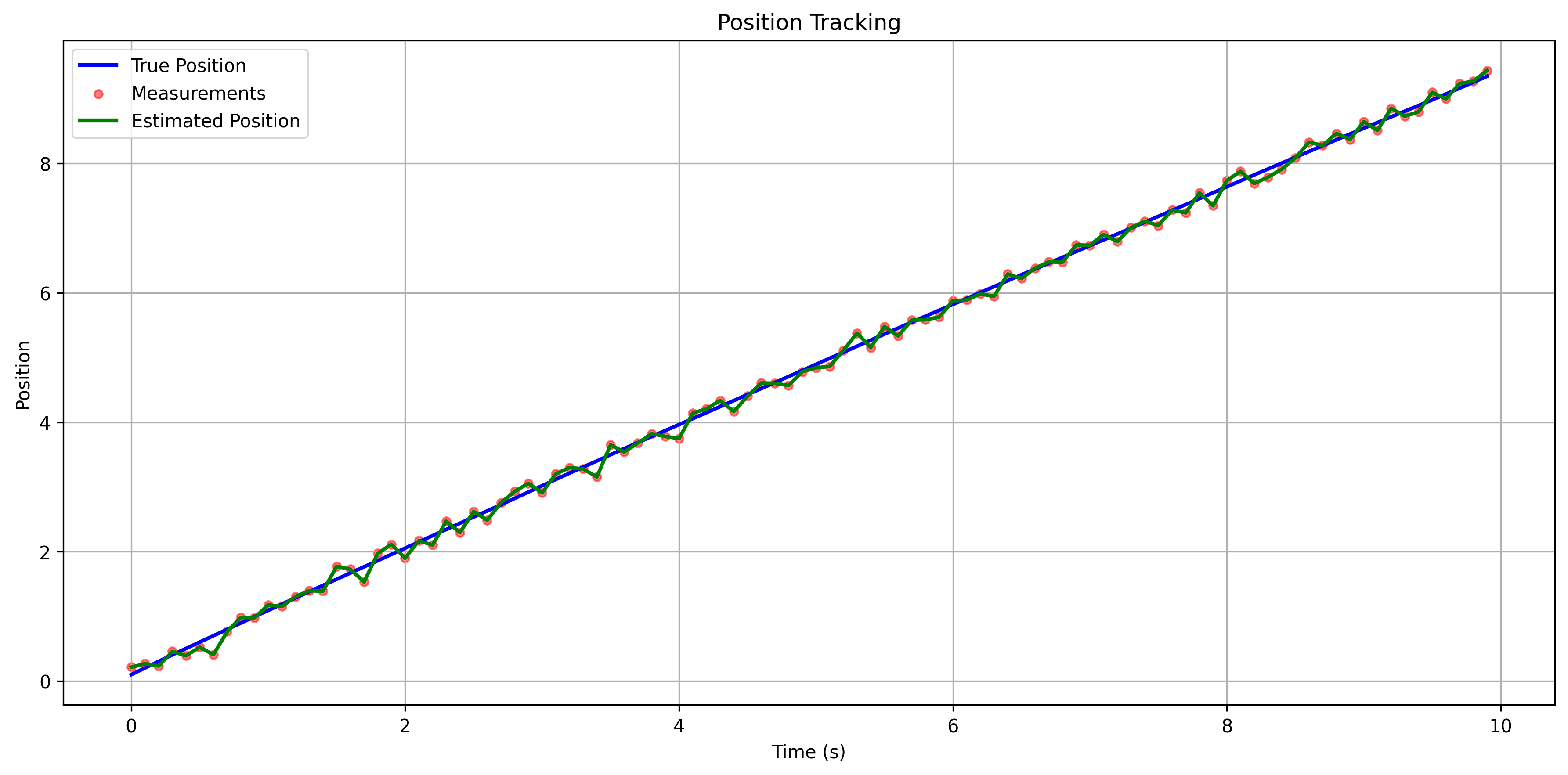
随着处理更多的测量值，估计值应该收敛到真实值，滤波器能有效降低测量噪声同时跟踪真实状态。

代码实现与结果可视化

代码实现

  1#include <stdio.h>
  2#include <math.h>
  3#include <gsl/gsl_matrix.h>
  4#include <gsl/gsl_blas.h>
  5#include <gsl/gsl_rng.h>
  6#include <gsl/gsl_randist.h>
  7
  8// 卡尔曼滤波器结构体
  9typedef struct
 10{
 11    gsl_matrix *A; // 状态转移矩阵
 12    gsl_matrix *H; // 观测矩阵
 13    gsl_matrix *Q; // 过程噪声协方差
 14    gsl_matrix *R; // 测量噪声协方差
 15    gsl_matrix *P; // 估计误差协方差
 16    gsl_matrix *K; // 卡尔曼增益
 17    gsl_matrix *x; // 状态向量 [位置, 速度]
 18} KalmanFilter;
 19
 20// 初始化卡尔曼滤波器
 21KalmanFilter *init_kalman_filter(double dt, double process_noise, double measurement_noise)
 22{
 23    KalmanFilter *kf = malloc(sizeof(KalmanFilter));
 24
 25    // 初始化矩阵
 26    kf->A = gsl_matrix_alloc(2, 2);
 27    kf->H = gsl_matrix_alloc(1, 2);
 28    kf->Q = gsl_matrix_alloc(2, 2);
 29    kf->R = gsl_matrix_alloc(1, 1);
 30    kf->P = gsl_matrix_alloc(2, 2);
 31    kf->K = gsl_matrix_alloc(2, 1);
 32    kf->x = gsl_matrix_alloc(2, 1);
 33
 34    // 设置状态转移矩阵 A
 35    gsl_matrix_set(kf->A, 0, 0, 1.0);
 36    gsl_matrix_set(kf->A, 0, 1, dt);
 37    gsl_matrix_set(kf->A, 1, 0, 0.0);
 38    gsl_matrix_set(kf->A, 1, 1, 1.0);
 39
 40    // 设置观测矩阵 H
 41    gsl_matrix_set(kf->H, 0, 0, 1.0);
 42    gsl_matrix_set(kf->H, 0, 1, 0.0);
 43
 44    // 设置过程噪声协方差 Q
 45    gsl_matrix_set(kf->Q, 0, 0, 0.25 * dt * dt * dt * dt * process_noise);
 46    gsl_matrix_set(kf->Q, 0, 1, 0.5 * dt * dt * dt * process_noise);
 47    gsl_matrix_set(kf->Q, 1, 0, 0.5 * dt * dt * dt * process_noise);
 48    gsl_matrix_set(kf->Q, 1, 1, dt * dt * process_noise);
 49
 50    // 设置测量噪声协方差 R
 51    gsl_matrix_set(kf->R, 0, 0, measurement_noise);
 52
 53    // 初始化估计误差协方差 P
 54    gsl_matrix_set_identity(kf->P);
 55    gsl_matrix_scale(kf->P, 1.0);
 56
 57    // 初始化状态向量
 58    gsl_matrix_set_zero(kf->x);
 59
 60    return kf;
 61}
 62
 63// 预测步骤
 64void predict(KalmanFilter *kf)
 65{
 66    // 临时矩阵
 67    gsl_matrix *temp_2x2 = gsl_matrix_alloc(2, 2);
 68    gsl_matrix *temp_2x1 = gsl_matrix_alloc(2, 1);
 69
 70    // x = A * x
 71    gsl_blas_dgemm(CblasNoTrans, CblasNoTrans, 1.0, kf->A, kf->x, 0.0, temp_2x1);
 72    gsl_matrix_memcpy(kf->x, temp_2x1);
 73
 74    // P = A * P * A' + Q
 75    gsl_blas_dgemm(CblasNoTrans, CblasTrans, 1.0, kf->A, kf->P, 0.0, temp_2x2);
 76    gsl_blas_dgemm(CblasNoTrans, CblasNoTrans, 1.0, temp_2x2, kf->A, 0.0, kf->P);
 77    gsl_matrix_add(kf->P, kf->Q);
 78
 79    // 释放临时矩阵
 80    gsl_matrix_free(temp_2x2);
 81    gsl_matrix_free(temp_2x1);
 82}
 83
 84// 更新步骤
 85void update(KalmanFilter *kf, double measurement)
 86{
 87    // 临时矩阵
 88    gsl_matrix *temp_1x2 = gsl_matrix_alloc(1, 2);   // For H*P
 89    gsl_matrix *temp_2x1 = gsl_matrix_alloc(2, 1);   // For P*H'
 90    gsl_matrix *temp_1x1 = gsl_matrix_alloc(1, 1);   // For H*x or innovation
 91    gsl_matrix *S = gsl_matrix_alloc(1, 1);          // Innovation covariance
 92    gsl_matrix *z = gsl_matrix_alloc(1, 1);          // Measurement
 93    gsl_matrix *innovation = gsl_matrix_alloc(1, 1); // z - H*x
 94
 95    // 设置测量值
 96    gsl_matrix_set(z, 0, 0, measurement);
 97
 98    // S = H * P * H' + R
 99    // First compute H*P (1x2 * 2x2 = 1x2)
100    gsl_blas_dgemm(CblasNoTrans, CblasNoTrans, 1.0, kf->H, kf->P, 0.0, temp_1x2);
101    // Then (H*P) * H' (1x2 * 2x1 = 1x1)
102    gsl_blas_dgemm(CblasNoTrans, CblasTrans, 1.0, temp_1x2, kf->H, 0.0, S);
103    gsl_matrix_add(S, kf->R);
104
105    // K = P * H' * S^(-1)
106    // First compute P*H' (2x2 * 2x1 = 2x1)
107    gsl_blas_dgemm(CblasNoTrans, CblasTrans, 1.0, kf->P, kf->H, 0.0, temp_2x1);
108    // Then scale by S^(-1)
109    double s_inv = 1.0 / gsl_matrix_get(S, 0, 0);
110    gsl_matrix_memcpy(kf->K, temp_2x1);
111    gsl_matrix_scale(kf->K, s_inv);
112
113    // 计算创新项 (innovation = z - H*x)
114    // First compute H*x (1x2 * 2x1 = 1x1)
115    gsl_blas_dgemm(CblasNoTrans, CblasNoTrans, 1.0, kf->H, kf->x, 0.0, temp_1x1);
116    gsl_matrix_memcpy(innovation, z);
117    gsl_matrix_sub(innovation, temp_1x1);
118
119    // x = x + K * innovation
120    // K*innovation (2x1 * 1x1 = 2x1)
121    gsl_blas_dgemm(CblasNoTrans, CblasNoTrans, 1.0, kf->K, innovation, 1.0, kf->x);
122
123    // P = (I - K*H) * P
124    // First compute K*H (2x1 * 1x2 = 2x2)
125    gsl_matrix *temp_2x2 = gsl_matrix_alloc(2, 2);
126    gsl_blas_dgemm(CblasNoTrans, CblasNoTrans, -1.0, kf->K, kf->H, 0.0, temp_2x2);
127    gsl_matrix_set_identity(temp_2x2); // Add identity matrix
128    // Then multiply by P
129    gsl_matrix *new_P = gsl_matrix_alloc(2, 2);
130    gsl_blas_dgemm(CblasNoTrans, CblasNoTrans, 1.0, temp_2x2, kf->P, 0.0, new_P);
131    gsl_matrix_memcpy(kf->P, new_P);
132
133    // 释放临时矩阵
134    gsl_matrix_free(temp_1x2);
135    gsl_matrix_free(temp_2x1);
136    gsl_matrix_free(temp_1x1);
137    gsl_matrix_free(temp_2x2);
138    gsl_matrix_free(new_P);
139    gsl_matrix_free(S);
140    gsl_matrix_free(z);
141    gsl_matrix_free(innovation);
142}
143
144// 释放卡尔曼滤波器
145void free_kalman_filter(KalmanFilter *kf)
146{
147    gsl_matrix_free(kf->A);
148    gsl_matrix_free(kf->H);
149    gsl_matrix_free(kf->Q);
150    gsl_matrix_free(kf->R);
151    gsl_matrix_free(kf->P);
152    gsl_matrix_free(kf->K);
153    gsl_matrix_free(kf->x);
154    free(kf);
155}
156
157int main()
158{
159    // 初始化随机数生成器
160    gsl_rng *rng = gsl_rng_alloc(gsl_rng_default);
161    gsl_rng_set(rng, 1234);
162
163    // 初始化卡尔曼滤波器参数
164    double dt = 0.1;                 // 时间步长
165    double process_noise = 0.01;     // 过程噪声
166    double measurement_noise = 0.01; // 测量噪声
167
168    // 创建卡尔曼滤波器
169    KalmanFilter *kf = init_kalman_filter(dt, process_noise, measurement_noise);
170
171    // 模拟数据
172    double true_position = 0.0;
173    double true_velocity = 1.0;
174
175    // 使用固定宽度格式化输出表头
176    printf("#%8s\t%8s\t%8s\t%8s\t%8s\t%8s\n",
177           "Time", "True Pos", "True Vel",
178           "Meas Pos",
179           "Est Pos", "Est Vel");
180
181    // 运行模拟
182    for (int t = 0; t < 100; t++)
183    {
184        // 加速度扰动考虑
185        true_velocity += gsl_ran_gaussian(rng, sqrt(process_noise)) * dt;
186
187        // 更新真实状态
188        true_position += true_velocity * dt;
189
190        // 生成带噪声的测量值
191        double measurement = true_position + gsl_ran_gaussian(rng, sqrt(measurement_noise));
192
193        // 卡尔曼滤波
194        predict(kf);
195        update(kf, measurement);
196
197        // 使用固定宽度格式化输出数据
198        printf("%9.2f\t%8.4f\t%8.4f\t%8.4f\t%8.4f\t%8.4f\n",
199               t * dt,
200               true_position,
201               true_velocity,
202               measurement,
203               gsl_matrix_get(kf->x, 0, 0),
204               gsl_matrix_get(kf->x, 1, 0));
205    }
206
207    // 清理
208    free_kalman_filter(kf);
209    gsl_rng_free(rng);
210
211    return 0;
212}

编译：

1gcc kalman.c -o kalman -lgsl -lgslcblas -lm

需要系统中安装了 gsl 库。安装方法：

1sudo apt-get install libgsl-dev

运行：

1./kalman > kalman_data.txt

就能看到一个文本文件 kalman_data.txt，里面记录了时间、真实位置、真实速度、测量位置、估计位置、估计速度。

结果可视化

很无聊的用Python做了一个可视化，直接从c代码生成可执行文件，然后捕获输出画图。

  1import subprocess
  2import numpy as np
  3import matplotlib.pyplot as plt
  4import os
  5
  6
  7def compile_kalman():
  8    """Compile the Kalman filter C program"""
  9    try:
 10        result = subprocess.run(
 11            ['gcc', 'kalman.c', '-o', 'kalman', '-lgsl', '-lgslcblas', '-lm'],
 12            capture_output=True,
 13            text=True
 14        )
 15        if result.returncode != 0:
 16            print("Error compiling kalman filter:")
 17            print(result.stderr)
 18            return False
 19        return True
 20    except Exception as e:
 21        print(f"Error during compilation: {e}")
 22        return False
 23
 24
 25def run_kalman_filter():
 26    """Run the Kalman filter executable and return the results"""
 27    try:
 28        # First compile the program
 29        if not compile_kalman():
 30            return None
 31
 32        # Run the executable and capture output
 33        result = subprocess.run(['./kalman'], capture_output=True, text=True)
 34
 35        # Clean up the executable
 36        try:
 37            os.remove('./kalman')
 38        except OSError as e:
 39            print(f"Warning: Could not remove executable: {e}")
 40
 41        if result.returncode != 0:
 42            print("Error running kalman filter executable")
 43            return None
 44
 45        # Parse the output
 46        lines = result.stdout.strip().split('\n')
 47
 48        # Skip the header line (starts with #)
 49        data = np.array([line.split()
 50                        for line in lines if not line.startswith('#')], dtype=float)
 51
 52        return data
 53    except Exception as e:
 54        print(f"Error: {e}")
 55        # Try to clean up if something went wrong
 56        try:
 57            os.remove('./kalman')
 58        except OSError:
 59            pass
 60        return None
 61
 62
 63def plot_position(data):
 64    """Plot position tracking results"""
 65    plt.figure(figsize=(12, 6))
 66
 67    time = data[:, 0]
 68    plt.plot(time, data[:, 1], 'b-', label='True Position', linewidth=2)
 69    plt.scatter(time, data[:, 3], c='r', s=20, alpha=0.5, label='Measurements')
 70    plt.plot(time, data[:, 4], 'g-', label='Estimated Position', linewidth=2)
 71
 72    plt.title('Position Tracking')
 73    plt.xlabel('Time (s)')
 74    plt.ylabel('Position')
 75    plt.grid(True)
 76    plt.legend()
 77
 78    plt.tight_layout()
 79    plt.savefig('kalman_filter_position.png', dpi=300, bbox_inches='tight')
 80    plt.close()
 81
 82
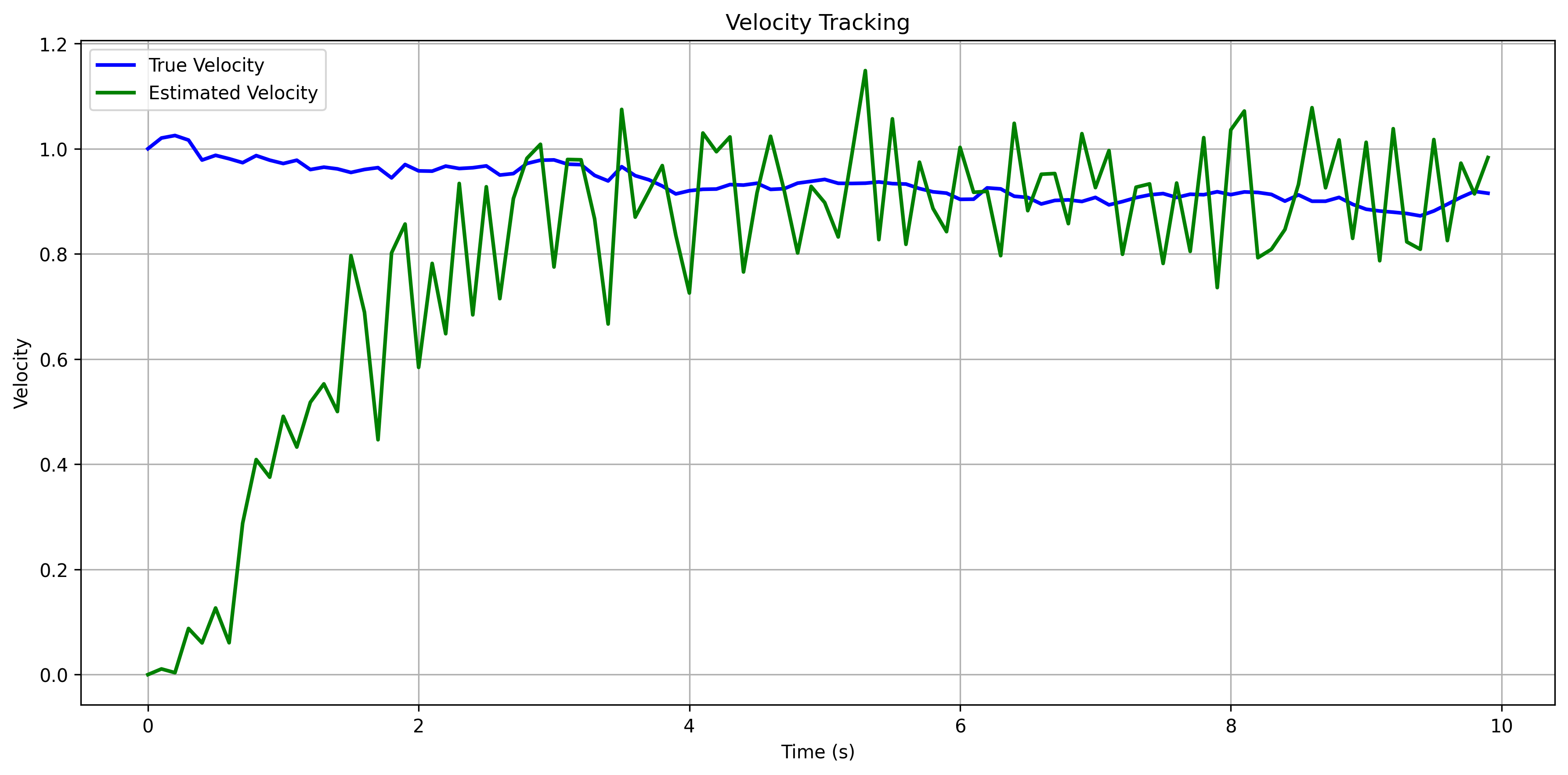
 83def plot_velocity(data):
 84    """Plot velocity tracking results"""
 85    plt.figure(figsize=(12, 6))
 86
 87    time = data[:, 0]
 88    plt.plot(time, data[:, 2], 'b-', label='True Velocity', linewidth=2)
 89    plt.plot(time, data[:, 5], 'g-', label='Estimated Velocity', linewidth=2)
 90
 91    plt.title('Velocity Tracking')
 92    plt.xlabel('Time (s)')
 93    plt.ylabel('Velocity')
 94    plt.grid(True)
 95    plt.legend()
 96
 97    plt.tight_layout()
 98    plt.savefig('kalman_filter_velocity.png', dpi=300, bbox_inches='tight')
 99    plt.close()
100
101
102def plot_results(data):
103    """Plot all results"""
104    plot_position(data)
105    plot_velocity(data)
106
107    # Create a combined plot for display
108    fig, (ax1, ax2) = plt.subplots(2, 1, figsize=(12, 10))
109    fig.suptitle('Kalman Filter Results', fontsize=16)
110
111    # Get time array
112    time = data[:, 0]
113
114    # Plot position tracking
115    ax1.plot(time, data[:, 1], 'b-', label='True Position', linewidth=2)
116    ax1.scatter(time, data[:, 3], c='r', s=20, alpha=0.5, label='Measurements')
117    ax1.plot(time, data[:, 4], 'g-', label='Estimated Position', linewidth=2)
118
119    ax1.set_title('Position Tracking')
120    ax1.set_xlabel('Time (s)')
121    ax1.set_ylabel('Position')
122    ax1.grid(True)
123    ax1.legend()
124
125    # Plot velocity tracking
126    ax2.plot(time, data[:, 2], 'b-', label='True Velocity', linewidth=2)
127    ax2.plot(time, data[:, 5], 'g-', label='Estimated Velocity', linewidth=2)
128
129    ax2.set_title('Velocity Tracking')
130    ax2.set_xlabel('Time (s)')
131    ax2.set_ylabel('Velocity')
132    ax2.grid(True)
133    ax2.legend()
134
135    # Adjust layout and display
136    plt.tight_layout()
137    plt.show()
138
139
140def main():
141    # Run Kalman filter and get data
142    data = run_kalman_filter()
143    if data is not None:
144        # Plot results
145        plot_results(data)
146    else:
147        print("Failed to get data from Kalman filter")
148
149
150if __name__ == "__main__":
151    main()

kalman_position

可以看到，我们从速度0开始，很快就追踪到速度1附近，然后速度估计基本就稳定在1附近了。

kalman_velocity